Multiple t-tests in R: One Test per Variable, All at Once

Q: How do I run a t-test on multiple variables at once in R?

Reshape your data from wide to long with tidyr::pivot_longer() so every measurement sits in one value column tagged by a variables column, then pipe into group_by(variables) %>% rstatix::t_test(value ~ group). Because the data is grouped, rstatix runs one t-test per variable and returns a single tidy data frame of results — no loop required.

Q: Should I adjust the p-values when testing many variables?

Yes. Running one t-test per variable is running a family of tests, so each carries its own chance of a false positive. Add adjust_pvalue(method = "BH") (Benjamini-Hochberg, controls the false-discovery rate) or method = "bonferroni" (stricter, controls the family-wise error rate) to your pipeline and report the resulting p.adj column rather than the raw p.

Q: What is the difference between t_test() and pairwise_t_test() in rstatix?

t_test() compares exactly two groups. pairwise_t_test() compares every pair of a factor’s levels, so use it when your grouping variable has three or more groups. Both slot into the same group_by(variables) %>% ... batch pattern; pairwise_t_test() simply returns several comparison rows per variable instead of one, with a built-in p.adjust.method argument.

Q: Does rstatix t_test() assume equal variances?

No — by default t_test() runs Welch’s t-test, which does not assume the two groups have equal variances (this is also R’s own t.test() default). Pass var.equal = TRUE if you specifically want the classic Student’s t-test that pools the variance.

Q: How do I add the p-values to a faceted ggplot?

Call add_xy_position(x = "Species") on your rstatix result to compute bracket coordinates, then add stat_pvalue_manual(stat.test, label = "p.adj.signif") to a ggpubr::ggboxplot() that is faceted with facet_wrap(~variables). rstatix places each variable’s bracket in the correct panel automatically; use label = "p.adj" to print the numeric adjusted p-value instead of the stars.

Reshape wide→long, then run and adjust a t-test for every outcome variable with rstatix

Biostatistics

Run a t-test across many outcome variables at once in R. Reshape wide→long with pivot_longer(), group by variable, and use rstatix t_test() to get one tidy test per variable — with p-values adjusted across the whole batch and a faceted ggpubr boxplot that prints the significance. Covers the two-group case and pairwise comparisons for a 3+ level factor.

Author

Alboukadel Kassambara

Published

July 13, 2026

Modified

July 12, 2026

What you’ll learn

The batch pattern — reshape wide→long with pivot_longer(), then run one t-test per outcome variable in a single pipeline.
rstatix t_test() — a tidy data frame of results (statistic, df, p) instead of a pile of t.test() printouts.
Adjust across the batch — adjust_pvalue() corrects the p-values for the many tests you just ran, so you don’t over-call significance.
Publication-grade plots — a faceted ggpubr boxplot with the significance printed on each panel via stat_pvalue_manual().
The pairwise angle — when your group has 3+ levels, swap in pairwise_t_test() to compare every pair, per variable.

You have a data frame with several outcome variables — say four flower measurements — and one grouping factor, and you want to know, for each variable, whether the two groups differ. Running t.test() by hand four times works, but it is tedious, error-prone, and leaves you with four console printouts you then have to read one at a time. Worse, four separate tests means four chances at a false positive, and nothing has corrected for that.

The tidy way is a batch workflow: reshape the data so every measurement lives in one column, run one t-test per variable in a single grouped pipeline, and get back a tidy table you can adjust, sort, and plot. This post shows that pattern with rstatix — a tidy wrapper around R’s classic tests — and ggpubr for the figure. A t-test compares the means of two groups; here we simply run one for every variable at once.

Setup

Load the tidyverse (for pivot_longer()), rstatix (for the tests), and ggpubr (for the plot):

library(tidyverse)
library(rstatix)
library(ggpubr)

We’ll use the built-in iris dataset. For the first, two-group example we drop the setosa species so we compare exactly two groups — versicolor vs. virginica — across the four measurements:

mydata <- iris %>%
  filter(Species != "setosa") %>%
  as_tibble()

head(mydata)

# A tibble: 6 × 5
  Sepal.Length Sepal.Width Petal.Length Petal.Width Species   
         <dbl>       <dbl>        <dbl>       <dbl> <fct>     
1          7           3.2          4.7         1.4 versicolor
2          6.4         3.2          4.5         1.5 versicolor
3          6.9         3.1          4.9         1.5 versicolor
4          5.5         2.3          4           1.3 versicolor
5          6.5         2.8          4.6         1.5 versicolor
6          5.7         2.8          4.5         1.3 versicolor

Reshape wide → long

The four measurements sit in four separate columns — that is wide format. To test them in one pass, stack them into a single value column tagged by a variables column. tidyr::pivot_longer() does exactly this:

mydata.long <- mydata %>%
  pivot_longer(
    -Species,                    # keep Species as-is; pivot everything else
    names_to = "variables",      # the old column names go here
    values_to = "value"          # their numbers go here
  )

head(mydata.long)

# A tibble: 6 × 3
  Species    variables    value
  <fct>      <chr>        <dbl>
1 versicolor Sepal.Length   7  
2 versicolor Sepal.Width    3.2
3 versicolor Petal.Length   4.7
4 versicolor Petal.Width    1.4
5 versicolor Sepal.Length   6.4
6 versicolor Sepal.Width    3.2

Every row is now one measurement: a species, which variable it is, and the value. This is the shape that lets group_by(variables) fan a test out over all four measurements at once.

Summary statistics per variable

Before testing, look at the numbers. rstatix’s get_summary_stats() gives a tidy n / mean / sd for each variable × group — the context you need to interpret any p-value:

mydata.long %>%
  group_by(variables, Species) %>%
  get_summary_stats(value, type = "mean_sd")

# A tibble: 8 × 6
  Species    variables    variable     n  mean    sd
  <fct>      <chr>        <fct>    <dbl> <dbl> <dbl>
1 versicolor Petal.Length value       50  4.26 0.47 
2 virginica  Petal.Length value       50  5.55 0.552
3 versicolor Petal.Width  value       50  1.33 0.198
4 virginica  Petal.Width  value       50  2.03 0.275
5 versicolor Sepal.Length value       50  5.94 0.516
6 virginica  Sepal.Length value       50  6.59 0.636
7 versicolor Sepal.Width  value       50  2.77 0.314
8 virginica  Sepal.Width  value       50  2.97 0.322

Already the story is visible: the two petal measurements separate the species cleanly (virginica’s petals are much larger), while Sepal.Width barely differs. The tests below just put numbers on that.

One t-test per variable

Here is the whole point. Group the long data by variables, then pipe into rstatix t_test(). Because the data is grouped, rstatix runs the test once within each group — one t-test per measurement — and returns a single tidy table:

stat.test <- mydata.long %>%
  group_by(variables) %>%
  t_test(value ~ Species) %>%
  adjust_pvalue(method = "BH") %>%
  add_significance()

stat.test

# A tibble: 4 × 11
  variables    .y.   group1 group2    n1    n2 statistic    df        p    p.adj
  <chr>        <chr> <chr>  <chr>  <int> <int>     <dbl> <dbl>    <dbl>    <dbl>
1 Petal.Length value versi… virgi…    50    50    -12.6   95.6 4.90e-22 9.80e-22
2 Petal.Width  value versi… virgi…    50    50    -14.6   89.0 2.11e-25 8.45e-25
3 Sepal.Length value versi… virgi…    50    50     -5.63  94.0 1.87e- 7 2.49e- 7
4 Sepal.Width  value versi… virgi…    50    50     -3.21  97.9 1.82e- 3 1.82e- 3
# ℹ 1 more variable: p.adj.signif <chr>

Read the pipeline top to bottom:

t_test(value ~ Species) — for each variable, compare value between the two species. By default this is Welch’s t-test (it does not assume equal variances), the safe choice when group spreads differ.
adjust_pvalue(method = "BH") — you just ran four tests, so the raw p column overstates your evidence. This adds a p.adj column that corrects for the multiple variables using Benjamini-Hochberg (controls the false-discovery rate). Use "bonferroni" for the stricter family-wise variant.
add_significance() — appends the familiar star column (p.adj.signif: ****, ***, **, *, ns) for quick scanning and for the plot labels.

The output is one row per variable with the estimate direction (statistic), the Welch degrees of freedom (df), the raw p, the adjusted p.adj, and the stars. All four measurements differ significantly between versicolor and virginica after adjustment — the petals overwhelmingly so (p.adj around 1e-22 to 1e-25), Sepal.Width the weakest (p.adj ≈ 0.0018, still **).

Adjust across the variables, not within

adjust_pvalue() here corrects across the four tests — one family of comparisons, one per outcome variable. That is the right correction when your question is “which of these variables differ between the two groups?” It is a different correction from adjusting within a variable across many group pairs, which is what the pairwise section below handles.

Visualize with a faceted boxplot

A table is precise; a figure is persuasive. Draw all four variables as faceted boxplots and print the adjusted significance on each panel. First call add_xy_position() so rstatix computes where each bracket should sit, then hand the result to stat_pvalue_manual():

set.seed(123)   # deterministic jitter positions across renders
stat.test <- stat.test %>%
  add_xy_position(x = "Species")

ggboxplot(
  mydata.long, x = "Species", y = "value",
  fill = "Species", palette = "npg", legend = "none",
  add = "jitter", add.params = list(size = 0.6, alpha = 0.4)
) +
  facet_wrap(~variables) +
  stat_pvalue_manual(stat.test, label = "p.adj.signif", tip.length = 0.01)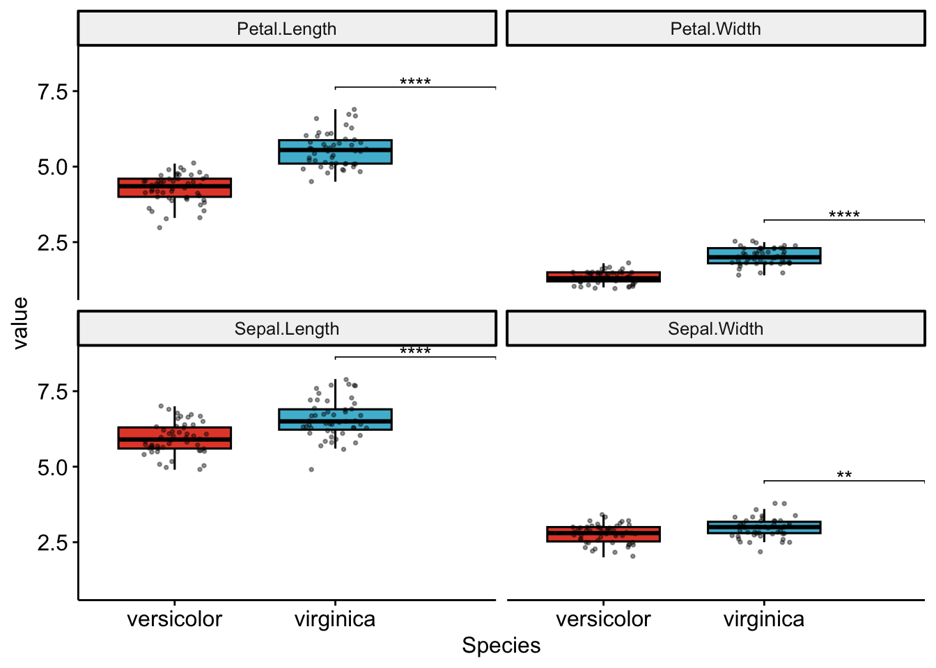

Faceted boxplots of four iris measurements comparing versicolor and virginica, each panel annotated with the Benjamini-Hochberg adjusted significance stars; petal measurements show four stars, sepal width two.

facet_wrap(~variables) gives each measurement its own panel; the npg (Nature Publishing Group) palette is a colourblind-safe journal scheme; the jittered points show the raw data behind each box; and stat_pvalue_manual() drops the adjusted stars exactly where add_xy_position() placed the bracket. One figure, four tests, fully annotated.

One plot per variable

Prefer a separate, individually-titled figure per variable (for a report or slide deck)? rstatix’s doo() applies a function within each group and stores the result — here a plot — in a list-column you can loop over:

graphs <- mydata.long %>%
  group_by(variables) %>%
  doo(
    ~ ggboxplot(
        data = ., x = "Species", y = "value",
        fill = "Species", palette = "npg", legend = "none"
      ),
    result = "plots"
  )

# Add the matching p-value to each and print
for (i in seq_along(graphs$variables)) {
  g <- graphs$plots[[i]] +
    labs(title = graphs$variables[i]) +
    stat_pvalue_manual(stat.test[i, ], label = "p.adj.signif")
  print(g)
}

Each element of graphs$plots is a standalone ggplot you can title, annotate with its own test row, and export separately — useful when the faceted grid is too small or you need one figure per file.

Pairwise comparisons for 3+ groups

The example above had exactly two groups. When your factor has three or more levels, a single t-test can’t compare them all — you want every pair of groups, per variable. Swap t_test() for pairwise_t_test() and keep the rest of the batch pattern identical. This time we use all three iris species:

iris.long <- iris %>%
  as_tibble() %>%
  pivot_longer(-Species, names_to = "variables", values_to = "value")

pwc <- iris.long %>%
  group_by(variables) %>%
  pairwise_t_test(value ~ Species, p.adjust.method = "bonferroni")

pwc

# A tibble: 12 × 10
   variables    .y.   group1     group2      n1    n2        p p.signif    p.adj
 * <chr>        <chr> <chr>      <chr>    <int> <int>    <dbl> <chr>       <dbl>
 1 Petal.Length value setosa     versico…    50    50 5.25e-69 ****     1.58e-68
 2 Petal.Length value setosa     virgini…    50    50 4.11e-91 ****     1.23e-90
 3 Petal.Length value versicolor virgini…    50    50 1.81e-31 ****     5.43e-31
 4 Petal.Width  value setosa     versico…    50    50 1.25e-57 ****     3.76e-57
 5 Petal.Width  value setosa     virgini…    50    50 7.95e-86 ****     2.39e-85
 6 Petal.Width  value versicolor virgini…    50    50 8.82e-37 ****     2.65e-36
 7 Sepal.Length value setosa     versico…    50    50 8.77e-16 ****     2.63e-15
 8 Sepal.Length value setosa     virgini…    50    50 2.21e-32 ****     6.64e-32
 9 Sepal.Length value versicolor virgini…    50    50 2.77e- 9 ****     8.30e- 9
10 Sepal.Width  value setosa     versico…    50    50 1.83e-17 ****     5.50e-17
11 Sepal.Width  value setosa     virgini…    50    50 4.54e-10 ****     1.36e- 9
12 Sepal.Width  value versicolor virgini…    50    50 3.15e- 3 **       9.44e- 3
# ℹ 1 more variable: p.adj.signif <chr>

For each of the four variables you now get three rows — setosa vs. versicolor, setosa vs. virginica, versicolor vs. virginica — with p.adjust.method = "bonferroni" correcting within each variable across its three pairwise comparisons. The plot follows the same recipe; add_xy_position() stacks the three brackets per panel automatically:

pwc <- pwc %>% add_xy_position(x = "Species")

ggboxplot(
  iris.long, x = "Species", y = "value",
  fill = "Species", palette = "npg", legend = "none"
) +
  facet_wrap(~variables) +
  stat_pvalue_manual(
    pwc, label = "p.adj.signif",
    tip.length = 0.01, step.increase = 0.06
  )

Faceted boxplots of four iris measurements across setosa, versicolor and virginica, each panel annotated with three Bonferroni-adjusted pairwise-comparison brackets and their significance stars.

Every species pair differs on every measurement (all ****) except versicolor vs. virginica on Sepal.Width, which is only ** — precisely the near-overlap the summary statistics hinted at.

Two different “pairwise” questions — don’t conflate them

This post runs a pairwise t-test across many variables — a batch of independent outcomes. That is different from pairwise comparisons between the levels of one factor as a post-hoc after ANOVA (Tukey HSD and friends), which is a curriculum topic in its own right. If you have a single outcome and one factor with several groups, do the ANOVA first, then its post-hoc — see the pairwise t-test lesson (and the ANOVA in R lesson for the omnibus test). Here, pairwise_t_test() is just the multi-level extension of the batch workflow.

Frequently asked questions

How do I run a t-test on multiple variables at once in R?

Reshape your data from wide to long with tidyr::pivot_longer() so every measurement sits in one value column tagged by a variables column, then pipe into group_by(variables) %>% rstatix::t_test(value ~ group). Because the data is grouped, rstatix runs one t-test per variable and returns a single tidy data frame of results — no loop required.

Should I adjust the p-values when testing many variables?

Yes. Running one t-test per variable is running a family of tests, so each carries its own chance of a false positive. Add adjust_pvalue(method = "BH") (Benjamini-Hochberg, controls the false-discovery rate) or method = "bonferroni" (stricter, controls the family-wise error rate) to your pipeline and report the resulting p.adj column rather than the raw p.

What is the difference between t_test() and pairwise_t_test() in rstatix?

t_test() compares exactly two groups. pairwise_t_test() compares every pair of a factor’s levels, so use it when your grouping variable has three or more groups. Both slot into the same group_by(variables) %>% ... batch pattern; pairwise_t_test() simply returns several comparison rows per variable instead of one, with a built-in p.adjust.method argument.

Does rstatix t_test() assume equal variances?

No — by default t_test() runs Welch’s t-test, which does not assume the two groups have equal variances (this is also R’s own t.test() default). Pass var.equal = TRUE if you specifically want the classic Student’s t-test that pools the variance.

How do I add the p-values to a faceted ggplot?

Call add_xy_position(x = "Species") on your rstatix result to compute bracket coordinates, then add stat_pvalue_manual(stat.test, label = "p.adj.signif") to a ggpubr::ggboxplot() that is faceted with facet_wrap(~variables). rstatix places each variable’s bracket in the correct panel automatically; use label = "p.adj" to print the numeric adjusted p-value instead of the stars.

Conclusion

Testing many outcome variables in R is not four copy-pasted t.test() calls — it’s one tidy pipeline: pivot_longer() to go long, group_by(variables) %>% t_test() (or pairwise_t_test() for 3+ groups) to fan the test out, adjust_pvalue() to correct for the batch, and a faceted ggpubr boxplot to show it. The result is reproducible, adjusted, and paper-ready — and the same pattern scales from four variables to forty.

Going deeper in /learn

For the reproducibility-gated, assumption-checked walkthroughs behind this batch pattern:

t-test in R — the one-sample, independent, and paired t-test in full, with normality and equal-variance checks and Cohen’s d effect size.
ANOVA in R — the right tool for one outcome across 3+ groups, plus the Tukey post-hoc pairwise comparisons.
Biostatistics — the full pillar, from comparing two groups to mixed models.

Citation

BibTeX citation:

@online{kassambara2026,
  author = {Kassambara, Alboukadel},
  title = {Multiple t-Tests in {R:} {One} {Test} Per {Variable,} {All}
    at {Once}},
  date = {2026-07-13},
  url = {https://www.datanovia.com/blog/multiple-t-tests-in-r-across-variables},
  langid = {en}
}

For attribution, please cite this work as:

Kassambara, Alboukadel. 2026. “Multiple t-Tests in R: One Test Per Variable, All at Once.” July 13. https://www.datanovia.com/blog/multiple-t-tests-in-r-across-variables.