3D Visualization in R with rgl: The Complete Guide
Build an interactive, rotatable 3D scene in R — scatter, spheres, axes, ellipses, a regression surface, and export
A complete, practical guide to 3D graphics in R with the rgl package: open a device, draw a 3D scatter with points3d and spheres3d, add axes and a bounding box, colour points by group, draw a 95% ellipse of concentration, fit a regression surface, and export a screenshot, a spinning GIF, or a self-contained interactive HTML widget. rgl renders through OpenGL, so this guide is static code plus real screenshots — run it locally to spin the scene yourself.
- A rotatable, interactive 3D scene in R with the
rglpackage — draw points and spheres, add axes and a bounding box, set the aspect ratio, and colour points by group. - The analytical extras that make a 3D scatter say something: a 95% ellipse of concentration (overall and per group) and a fitted regression surface.
- Three ways to share the result: a static PNG screenshot, a spinning GIF (
movie3d), and a self-contained interactive HTML widget (rglwidget). - Every figure below is a real screenshot of the code that produced it. Because
rgldraws through OpenGL, you run the code locally to get the live, spinnable scene.
rgl is R’s package for real-time interactive 3D graphics. It opens a hardware-accelerated window you can rotate with the mouse, zoom with the scroll wheel, and select regions in — the natural home for a 3D scatter plot where a fixed viewing angle always hides some points behind others. It renders through OpenGL (the cross-platform graphics library your GPU speaks), which is exactly why it’s so fluid on your own machine and why this guide ships as static screenshots: the live scene lives in an OpenGL window, not on a web page. Copy any block, run it in your R session, and drag to explore. See the rgl package on CRAN and the rgl reference site for the full API.
The figures here are screenshots captured from a local rgl session. There is no in-browser sandbox on this page — copy any block and run it in your own R session (after the short setup below) to reproduce each scene and rotate it yourself.
Older rgl tutorials (this one’s ancestor included) use the low-level rgl.* device functions — rgl.open(), rgl.points(), rgl.spheres(), rgl.bg(). Recent rgl versions deprecate these in favour of the higher-level R3D interface — open3d(), points3d(), spheres3d(), bg3d() — which handle materials and scenes more consistently. The two produce the same pictures, and we show the classic device calls because they map one-to-one to the screenshots, but for new code prefer the *3d functions. The mapping is direct: rgl.open → open3d, rgl.points → points3d, rgl.spheres → spheres3d, rgl.bg → bg3d, rgl.lines → segments3d, rgl.texts → text3d, rgl.bbox → bbox3d. The dedicated R3D interface section below uses the modern style throughout.
Install and load rgl
Install once from CRAN, then load it in each session:
install.packages("rgl")
library("rgl")
On Linux you may need the system OpenGL headers first (for example sudo apt-get install r-cran-rgl on Debian/Ubuntu, which pulls in the required libraries).
The data
Every example uses the built-in iris data — 150 flowers from three species (setosa, versicolor, virginica), measured on four variables. We plot three of them, storing the coordinates in x, y, z so the calls stay short:
data(iris)
x <- iris$Sepal.Length
y <- iris$Petal.Length
z <- iris$Sepal.Width
Open and close the device
An rgl scene lives in a device — its interactive window. A handful of functions manage it: open3d() (or the classic rgl.open()) opens a new one, rgl.close() closes the current device, rgl.clear() empties the current scene so you can redraw, and rgl.cur() returns the active device’s ID. In the first sections we open a fresh device per plot; further down, a small helper does it for us.
A basic 3D scatter plot
rgl.points() (modern: points3d()) draws the raw scatter. Open a device and hand it the three coordinate vectors:
rgl.open()                                  # Open a new RGL device
rgl.points(x, y, z, color = "lightgray")    # 3D scatter plot
The points are tiny and the background is dark by default. rgl.bg() (modern: bg3d()) sets the background colour, and size enlarges the markers:
rgl.open()                                       # Open a new RGL device
rgl.bg(color = "white")                          # White background
rgl.points(x, y, z, color = "blue", size = 5)    # Bigger blue points
rgl.viewpoint(zoom = 0.7)                         # Zoom in a little
Spheres instead of points
For a more three-dimensional feel, draw spheres with rgl.spheres() (modern: spheres3d()). The radius (here r) controls their size:
rgl.open()
rgl.bg(color = "white")
rgl.spheres(x, y, z, r = 0.2, color = "grey")
rgl.viewpoint(zoom = 0.7)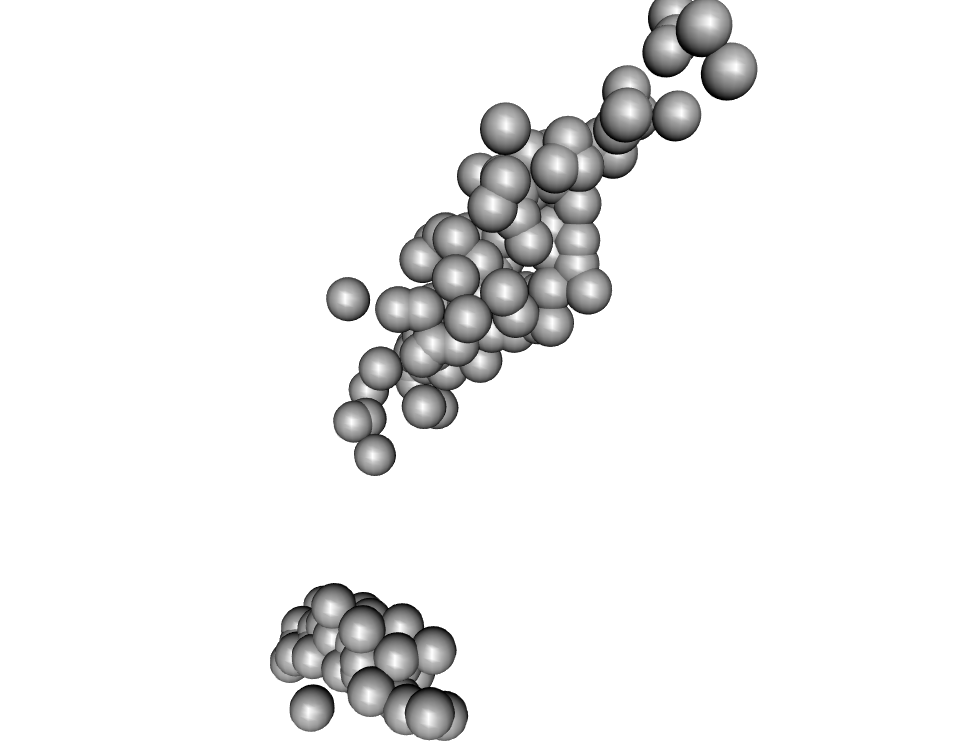
Remember the payoff of rgl: hold down the mouse to rotate the cloud and scroll to zoom. A single screenshot can’t show that a group hides behind another — rotating can.
A helper to initialize the device
Re-typing the same setup gets old. This small rgl_init() opens a device only when needed, sets a sensible window size, background, and viewpoint, and clears any previous shapes — so every later block starts from a clean, consistently-oriented scene:
rgl_init <- function(new.device = FALSE, bg = "white", width = 640) {
  if (new.device | rgl.cur() == 0) {
    rgl.open()
    par3d(windowRect = 50 + c(0, 0, width, width))   # Set the window size
    rgl.bg(color = bg)                               # Background colour
  }
  rgl.clear(type = c("shapes", "bboxdeco"))          # Clear the scene
  rgl.viewpoint(theta = 15, phi = 20, zoom = 0.7)    # Set the viewpoint
}
par3d(windowRect = ...) sizes the window, and rgl.viewpoint(theta, phi, zoom) fixes the camera — theta and phi are the polar angles, zoom the zoom factor. Setting the viewpoint in code just gives every screenshot the same angle; the scene stays fully interactive.
Add a bounding box
A bounding box frames the cloud and carries the scale. rgl.bbox() (modern: bbox3d()) draws it, and its material arguments style it:
rgl_init()
rgl.spheres(x, y, z, r = 0.2, color = "yellow")
# Styled bounding box with tick labels
rgl.bbox(color = c("#333377", "black"), emission = "#333377",
         specular = "#3333FF", shininess = 5, alpha = 0.8)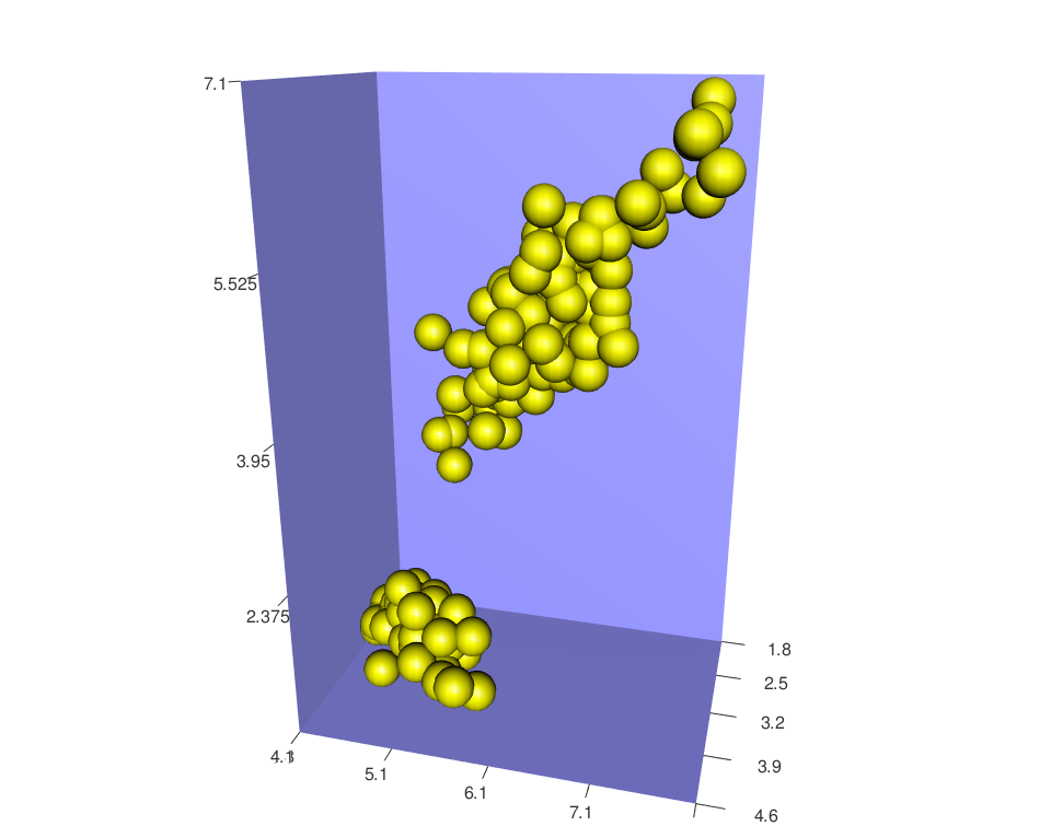
The first colour is the box’s background, the second the tick-label colour; alpha sets its transparency (0 fully transparent, 1 opaque). Arguments xlen, ylen, zlen control how many tick marks each axis gets.
Add axis lines and labels
To draw axes by hand, rgl.lines() (modern: segments3d()) draws a segment between two points and rgl.texts() (modern: text3d()) labels it. Passing each axis its data range looks natural until you notice the axes don’t meet at the origin:
rgl_init()
rgl.spheres(x, y, z, r = 0.2, color = "yellow")
# One coloured line per axis, spanning that variable's range
rgl.lines(c(min(x), max(x)), c(0, 0), c(0, 0), color = "black")
rgl.lines(c(0, 0), c(min(y), max(y)), c(0, 0), color = "red")
rgl.lines(c(0, 0), c(0, 0), c(min(z), max(z)), color = "green")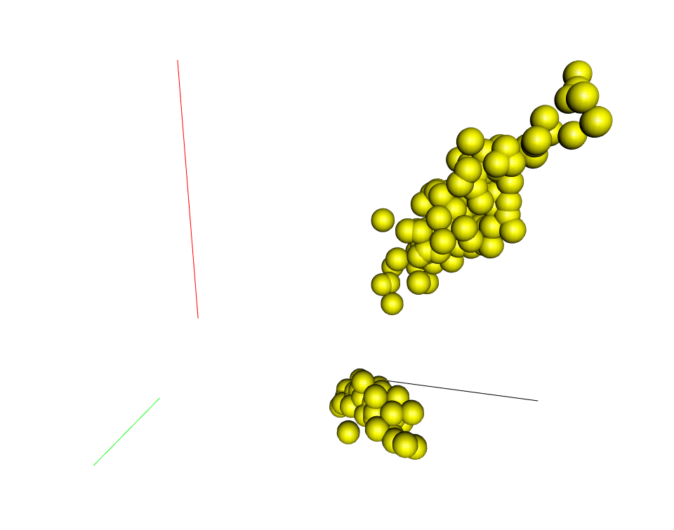
The fix is to build the axes around zero. This rgl_add_axes() helper spans each axis symmetrically with c(-max, max), marks the direction, labels it, and optionally adds a floor plane and a bounding box:
rgl_add_axes <- function(x, y, z, axis.col = "grey",
                         xlab = "", ylab = "", zlab = "", show.plane = TRUE,
                         show.bbox = FALSE, bbox.col = c("#333377", "black")) {
  lim <- function(x) c(-max(abs(x)), max(abs(x))) * 1.1
  # Axis lines through the origin
  xlim <- lim(x); ylim <- lim(y); zlim <- lim(z)
  rgl.lines(xlim, c(0, 0), c(0, 0), color = axis.col)
  rgl.lines(c(0, 0), ylim, c(0, 0), color = axis.col)
  rgl.lines(c(0, 0), c(0, 0), zlim, color = axis.col)
  # A point + label at the far end of each axis
  axes <- rbind(c(xlim[2], 0, 0), c(0, ylim[2], 0), c(0, 0, zlim[2]))
  rgl.points(axes, color = axis.col, size = 3)
  rgl.texts(axes, text = c(xlab, ylab, zlab), color = axis.col,
            adj = c(0.5, -0.8), size = 2)
  # Optional floor plane
  if (show.plane)
    rgl.quads(x = rep(xlim / 1.1, each = 2), y = c(0, 0, 0, 0),
              z = c(zlim[1], zlim[2], zlim[2], zlim[1]) / 1.1)
  # Optional bounding box
  if (show.bbox)
    rgl.bbox(color = c(bbox.col[1], bbox.col[2]), alpha = 0.5,
             emission = bbox.col[1], specular = bbox.col[1], shininess = 5,
             xlen = 3, ylen = 3, zlen = 3)
}
rgl.quads() (modern: quads3d()) draws the floor plane from the coordinates of its four corners. Now the axes cross cleanly at the origin:
rgl_init()
rgl.spheres(x, y, z, r = 0.2, color = "yellow")
rgl_add_axes(x, y, z)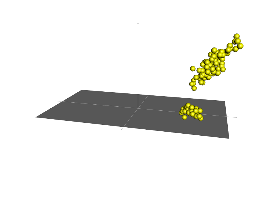
For readable scales, the simplest route is to let the bounding box carry the tick marks — pass show.bbox = TRUE:
rgl_init()
rgl.spheres(x, y, z, r = 0.2, color = "yellow")
rgl_add_axes(x, y, z, show.bbox = TRUE)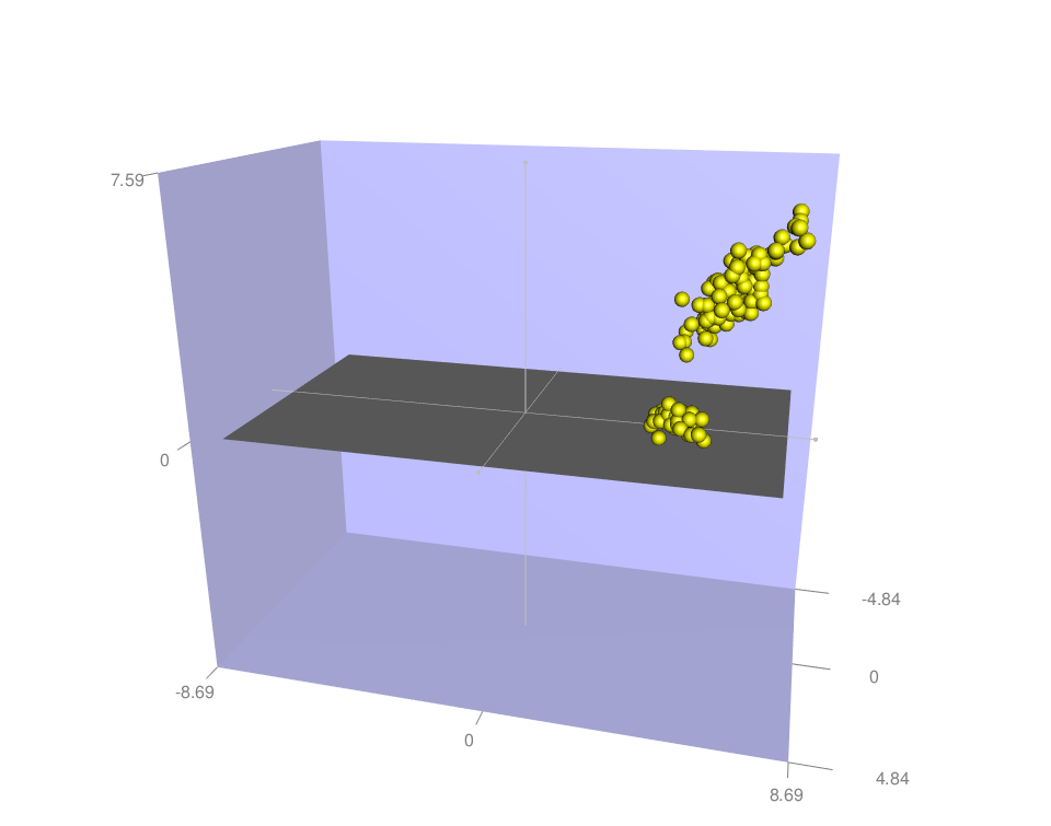
Set the aspect ratio
aspect3d() sets the apparent ratio of the three axes. With aspect3d(1, 1, 1) the bounding box is a cube, so all three variables are shown at the same visual scale (isometric — the default is aspect3d("iso")):
rgl_init()
rgl.spheres(x, y, z, r = 0.2, color = "yellow")
rgl_add_axes(x, y, z, show.bbox = TRUE)
aspect3d(1, 1, 1)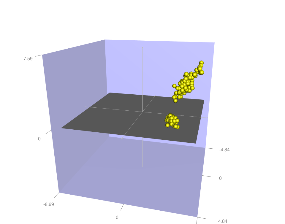
Change the ratios to stretch one axis — handy to spread out a cramped dimension. aspect3d(2, 1, 1) doubles the x-axis:
rgl_init()
rgl.spheres(x, y, z, r = 0.2, color = "yellow")
rgl_add_axes(x, y, z, show.bbox = TRUE)
aspect3d(2, 1, 1)   # Stretch the x axis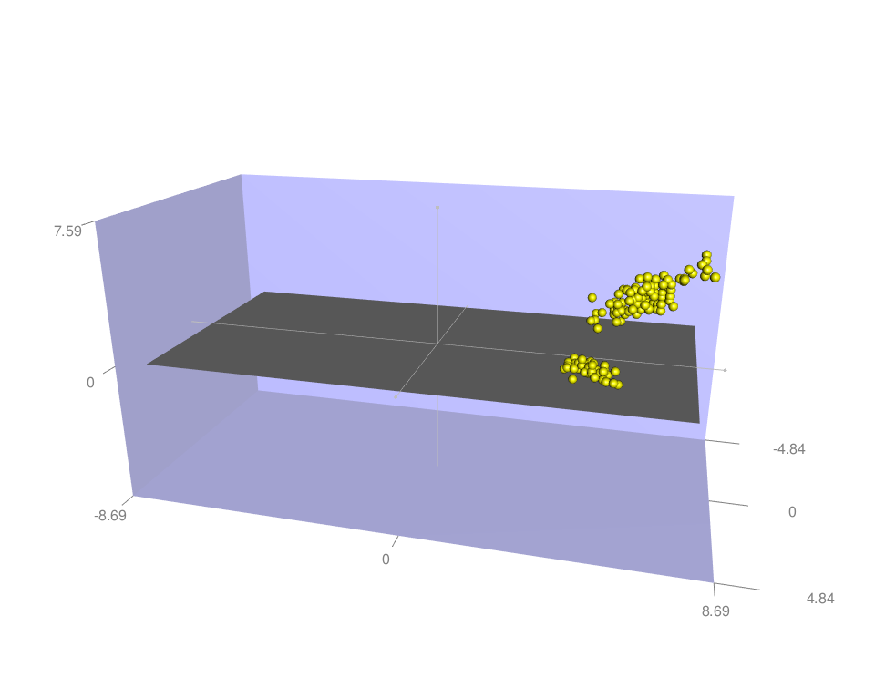
Colour points by group
The whole point of a 3D scatter is usually to see whether groups separate. A tiny helper turns a factor into a per-point colour vector — index a palette by the group number so each observation gets its group’s colour:
get_colors <- function(groups, group.col = palette()) {
  groups <- as.factor(groups)
  ngrps <- length(levels(groups))
  if (ngrps > length(group.col)) group.col <- rep(group.col, ngrps)
  color <- group.col[as.numeric(groups)]
  names(color) <- as.vector(groups)
  color
}
Pass its output straight to rgl.spheres():
rgl_init()
rgl.spheres(x, y, z, r = 0.2, color = get_colors(iris$Species))
rgl_add_axes(x, y, z, show.bbox = TRUE)
aspect3d(1, 1, 1)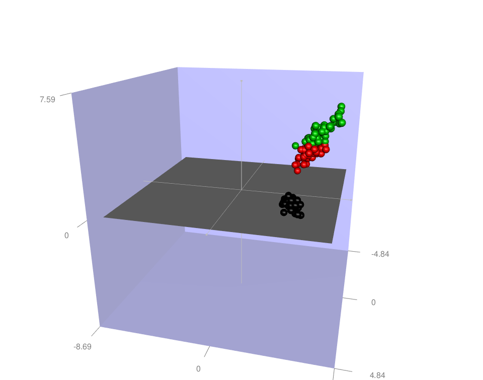
setosa clearly separates from the other two. Supply your own palette — a colourblind-safe one here — as the second argument:
cols <- get_colors(iris$Species, c("#999999", "#E69F00", "#56B4E9"))
rgl_init()
rgl.spheres(x, y, z, r = 0.2, color = cols)
rgl_add_axes(x, y, z, show.bbox = TRUE)
aspect3d(1, 1, 1)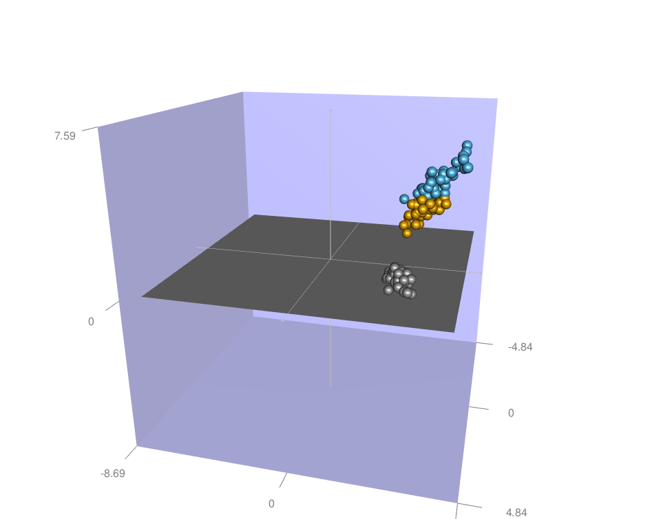
Or draw a palette from RColorBrewer — Dark2 is a solid qualitative choice:
library("RColorBrewer")
cols <- get_colors(iris$Species, brewer.pal(n = 3, name = "Dark2"))
rgl_init()
rgl.spheres(x, y, z, r = 0.2, color = cols)
rgl_add_axes(x, y, z, show.bbox = TRUE)
aspect3d(1, 1, 1)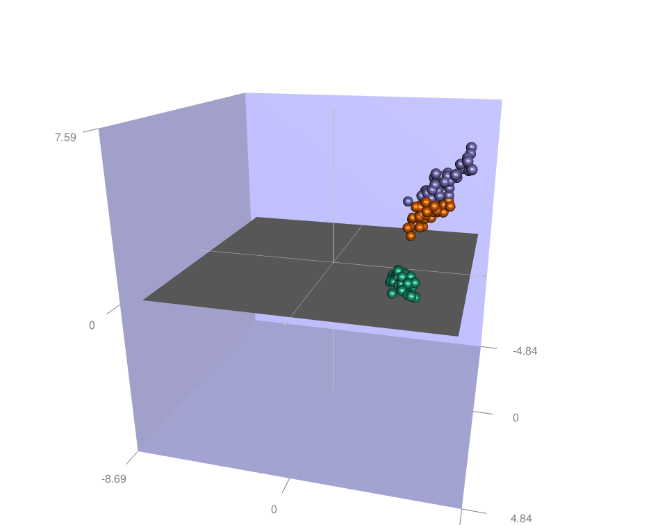
Choosing colours well is a topic of its own — see the R color palettes reference for the full catalog and when to reach for each type.
Change the shape of points
rgl ships six mesh objects — 3D solids you can use as markers: cube3d(), tetrahedron3d(), octahedron3d(), icosahedron3d(), dodecahedron3d(), and cuboctahedron3d().
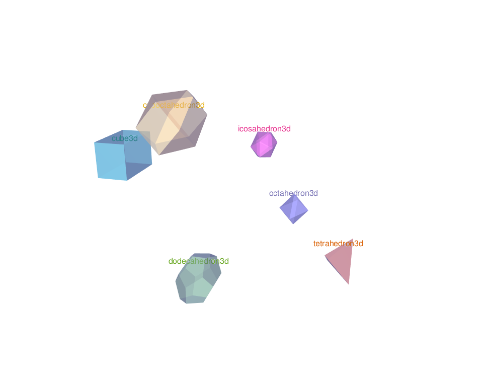
shapelist3d() places a chosen solid at each data point. Here tetrahedra stand in for spheres, coloured by species:
rgl_init()
shapelist3d(tetrahedron3d(), x, y, z, size = 0.15,
            color = get_colors(iris$Species))
rgl_add_axes(x, y, z, show.bbox = TRUE)
aspect3d(1, 1, 1)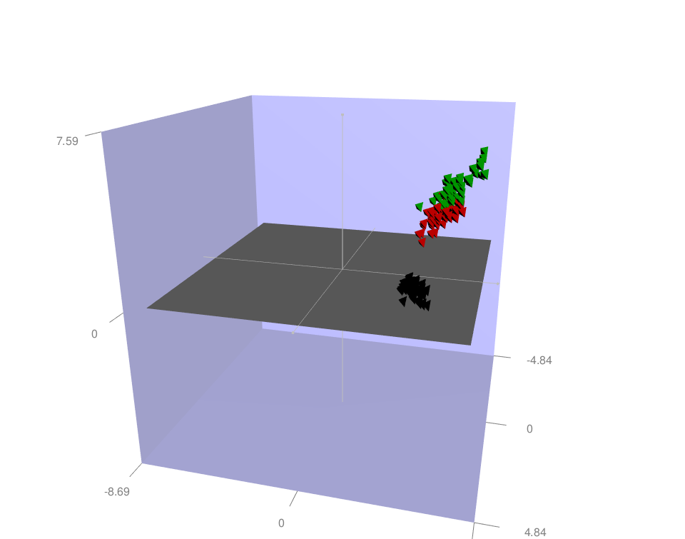
Add an ellipse of concentration
An ellipse of concentration (an ellipsoid, in 3D) is the region expected to contain a given fraction of the points under a normal model — the 3D cousin of a confidence ellipse. ellipse3d() estimates it from the covariance matrix; it returns a mesh3d object (rgl’s triangle-mesh geometry) that you draw with shade3d() (a solid surface), wire3d() (a wireframe), or both:
rgl_init()
rgl.spheres(x, y, z, r = 0.2, color = "#D95F02")
rgl_add_axes(x, y, z, show.bbox = TRUE)
# 95% ellipse of concentration
ellips <- ellipse3d(cov(cbind(x, y, z)),
                    centre = c(mean(x), mean(y), mean(z)), level = 0.95)
shade3d(ellips, col = "#D95F02", alpha = 0.1, lit = FALSE)   # translucent solid
wire3d(ellips, col = "#D95F02", lit = FALSE)                 # wireframe
aspect3d(1, 1, 1)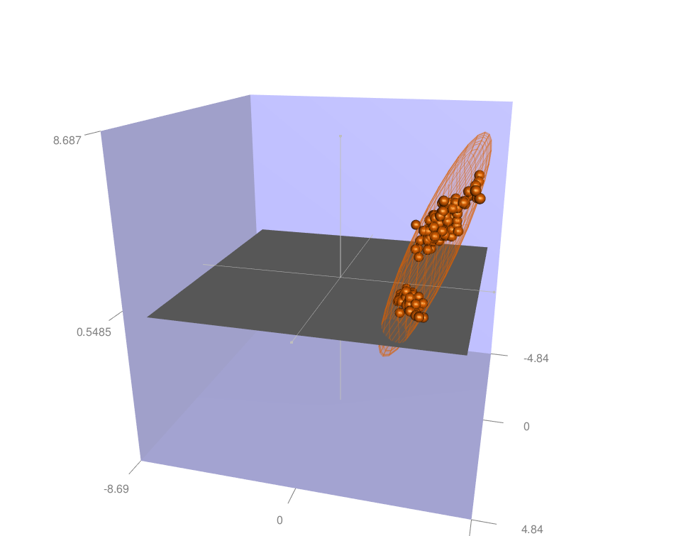
More useful is one ellipse per group — it shows each species’ spread and where they overlap. Loop over the levels, compute an ellipsoid from that group’s covariance, and label it at its centre:
groups <- iris$Species
levs <- levels(groups)
group.col <- c("red", "green", "blue")

rgl_init()
rgl.spheres(x, y, z, r = 0.2, color = group.col[as.numeric(groups)])
rgl_add_axes(x, y, z, show.bbox = FALSE)

for (i in seq_along(levs)) {
  selected <- groups == levs[i]
  xx <- x[selected]; yy <- y[selected]; zz <- z[selected]
  ellips <- ellipse3d(cov(cbind(xx, yy, zz)),
                      centre = c(mean(xx), mean(yy), mean(zz)), level = 0.95)
  shade3d(ellips, col = group.col[i], alpha = 0.1, lit = FALSE)
  texts3d(mean(xx), mean(yy), mean(zz), text = levs[i],
          col = group.col[i], cex = 2)   # label at the group centre
}
aspect3d(1, 1, 1)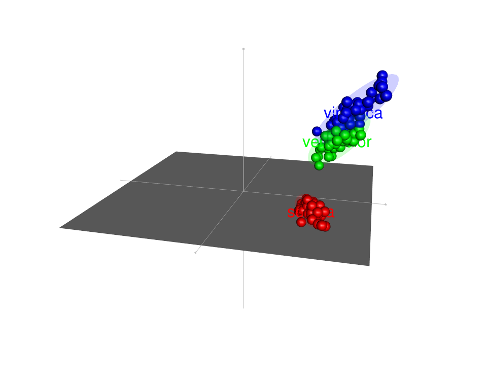
Fit a regression surface
To show how one variable depends on two others, fit a linear model and draw its surface. Predict the fitted values over a regular grid, then draw the grid with rgl.surface() (modern: surface3d()) — once filled, once as grid lines:
rgl_init()
rgl.spheres(x, y, z, r = 0.2, color = "#D95F02")
rgl_add_axes(x, y, z, show.bbox = FALSE)
aspect3d(1, 1, 1)

# Fit y ~ x + z and predict on a regular x-z grid
fit <- lm(y ~ x + z)
grid.lines <- 26
x.pred <- seq(min(x), max(x), length.out = grid.lines)
z.pred <- seq(min(z), max(z), length.out = grid.lines)
xz <- expand.grid(x = x.pred, z = z.pred)
y.pred <- matrix(predict(fit, newdata = xz), nrow = grid.lines, ncol = grid.lines)

# Draw the fitted surface, then its grid lines
rgl.surface(x.pred, z.pred, y.pred, color = "steelblue", alpha = 0.5, lit = FALSE)
rgl.surface(x.pred, z.pred, y.pred, color = "black", alpha = 0.5, lit = FALSE,
            front = "lines", back = "lines")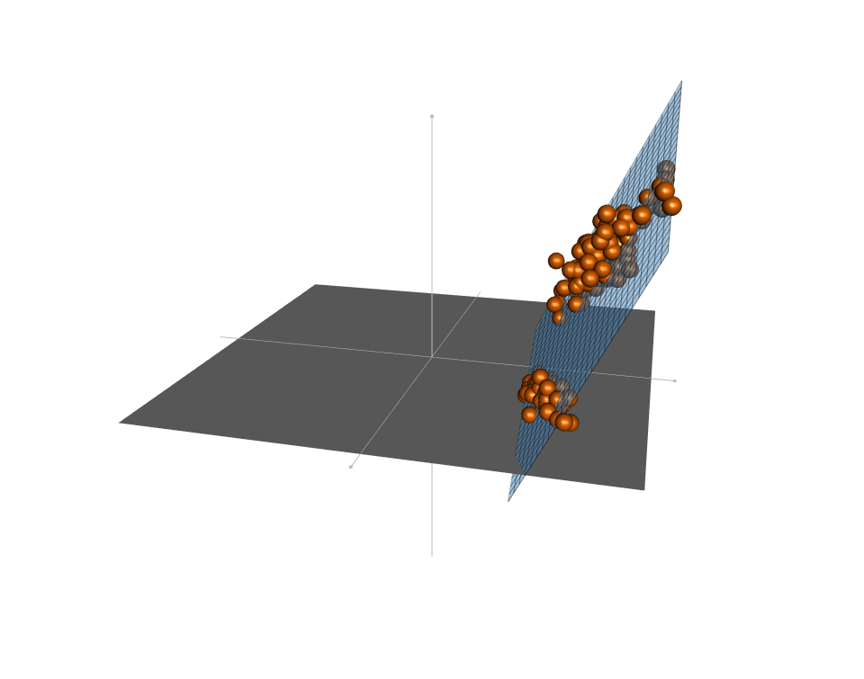
Points above the surface are under-predicted by the model, points below it over-predicted. (planes3d() draws a flat plane from the equation ax + by + cz + d = 0 if you only need the plane itself.)
The R3D interface: plot3d()
Everything above uses the low-level device functions. rgl also offers a higher-level R3D interface that feels like base R’s plot() — and it’s the recommended modern style. plot3d() draws the whole scatter in one call; type = "s" gives spheres, radius sizes them, and xlab/ylab/zlab label the axes:
open3d()
plot3d(x, y, z, col = "blue", box = FALSE, type = "s", radius = 0.15,
       xlab = "Sepal.Length", ylab = "Petal.Length", zlab = "Sepal.Width")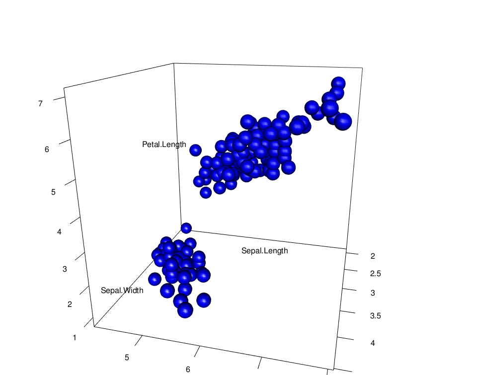
plot3d() also adds an ellipsoid directly — draw the scatter, compute the ellipse, and add it with type = "wire" for a clean cage:
open3d()
plot3d(x, y, z, col = "blue", box = FALSE, type = "s", radius = 0.15)
ellips <- ellipse3d(cov(cbind(x, y, z)),
                    centre = c(mean(x), mean(y), mean(z)), level = 0.95)
plot3d(ellips, col = "blue", alpha = 0.5, add = TRUE, type = "wire")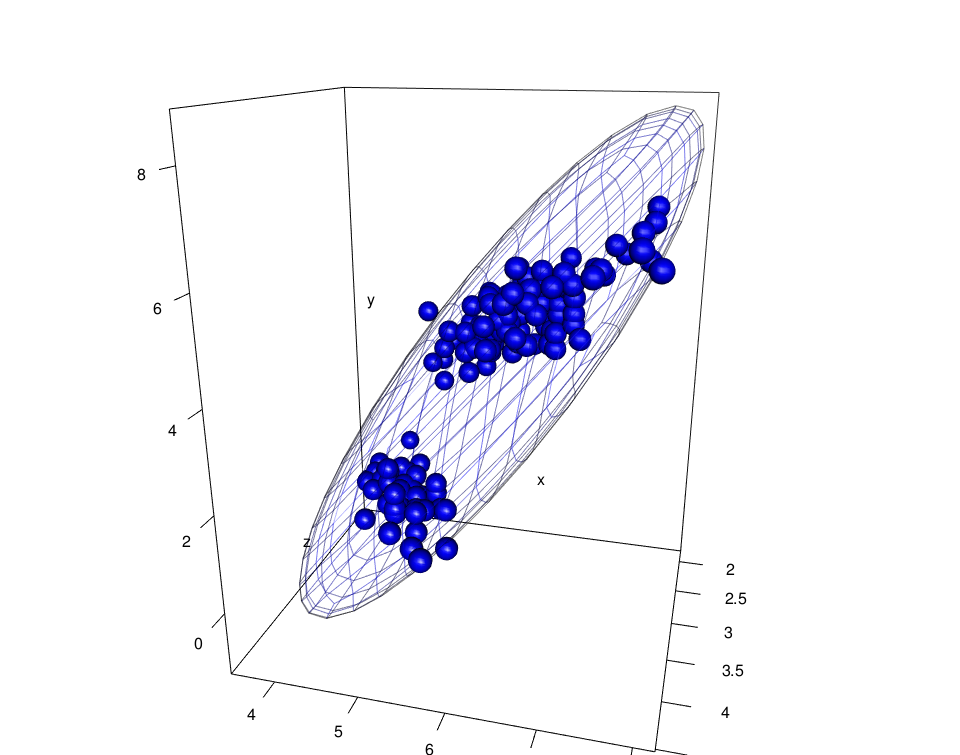
The R3D interface has a full set of “add a shape to the current scene” verbs — points3d(), lines3d(), segments3d(), quads3d(), text3d(), plus axes3d(), title3d(), and box3d() for decoration. This is the vocabulary to reach for in new rgl code.
Export your scene
Once the scene looks right, save it three ways.
A static image. snapshot3d() (classic: rgl.snapshot()) writes a PNG; postscript3d() (classic: rgl.postscript()) writes vector formats (PDF, SVG, EPS, …):
snapshot3d(filename = "plot.png")           # PNG screenshot
postscript3d("plot.pdf", fmt = "pdf")       # Vector PDF
A spinning GIF. movie3d() renders a rotation to an animated GIF (it needs ImageMagick installed for the GIF conversion). spin3d() supplies the rotation:
movie3d(spin3d(axis = c(0, 0, 1)), duration = 3, dir = getwd())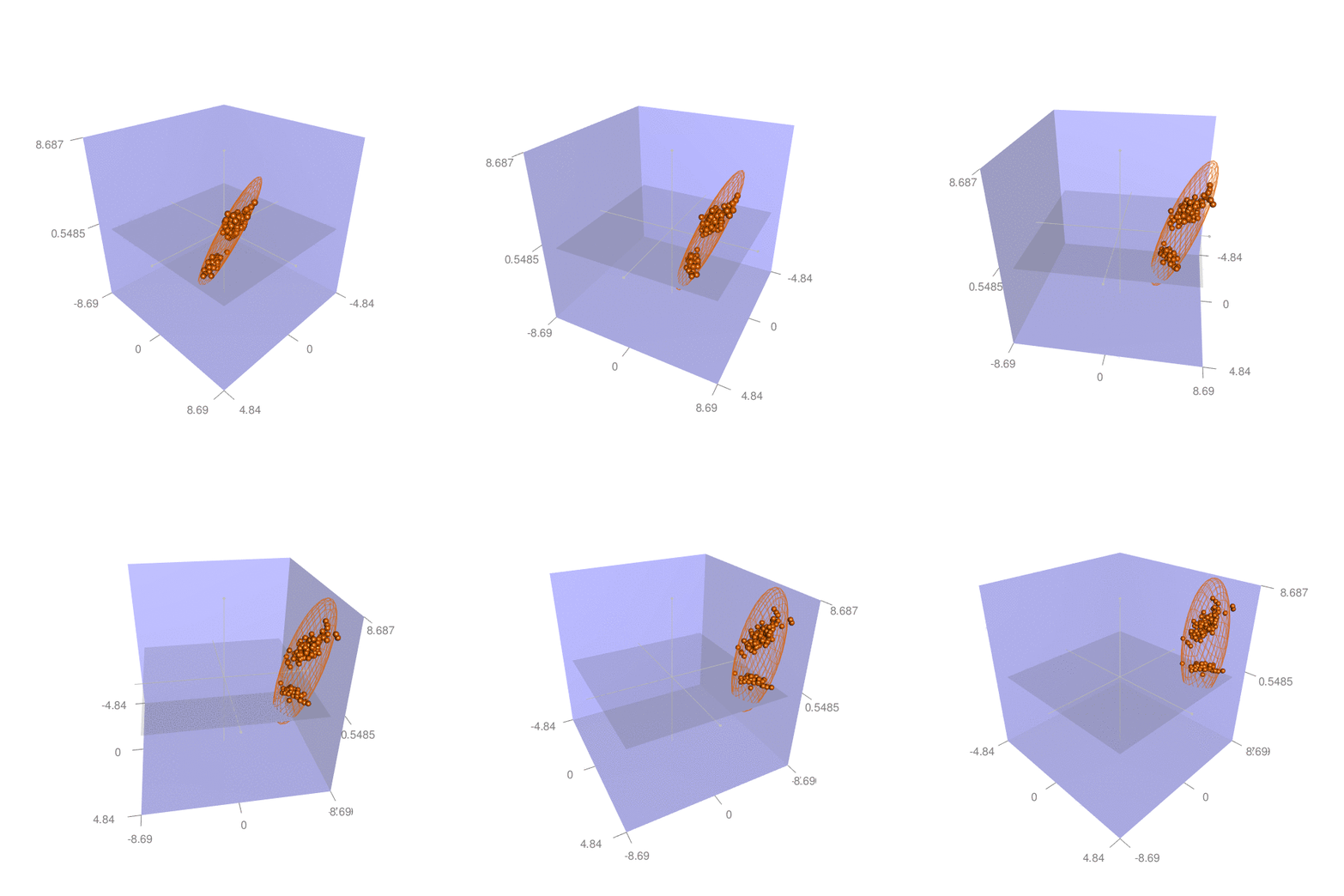
An interactive HTML widget. To keep the interactivity on a web page, export the scene with rglwidget() and save it with htmlwidgets::saveWidget(). This is the modern replacement for the old writeWebGL() (which was removed from recent rgl), and it produces a self-contained, rotatable WebGL page — WebGL is the browser’s version of OpenGL:
open3d()
plot3d(x, y, z, col = get_colors(iris$Species), type = "s", radius = 0.15)
# Save the current scene as a stand-alone interactive HTML page
htmlwidgets::saveWidget(rglwidget(), file = "rgl-scene.html")
Select and identify points
Because the scene is live, you can also pick points with the mouse. select3d() returns a test function for a region you drag out; identify3d() labels points you click — both are interactive, so they run in your local session (there’s no static screenshot to show):
# Drag a box to select points, then recolour them
f <- select3d()
sel <- f(x, y, z)
rgl.spheres(x[sel], y[sel], z[sel], r = 0.2, color = "green")

# Or click to label up to 5 points
identify3d(x, y, z, labels = rownames(iris), n = 5)
Frequently asked questions
rgl builds real-time interactive 3D graphics in R through OpenGL. You can draw 3D scatter plots, spheres, surfaces, meshes and ellipsoids, then rotate the scene with the mouse, zoom with the scroll wheel, and select points. It’s the go-to for 3D scatter plots where a single fixed angle would hide points behind one another, and it can export a static screenshot, a spinning GIF, or a self-contained interactive HTML widget.
Install and load rgl, then use the R3D interface: plot3d(x, y, z, type = "s", radius = 0.15, col = "blue"). It opens a hardware-accelerated window you can drag to rotate and scroll to zoom. Colour by group by passing a per-point colour vector to col, and add a decoration such as a bounding box (bbox3d()) or a concentration ellipsoid (ellipse3d()).
rgl renders through an OpenGL window, which doesn’t embed as a static image on its own. To put an rgl scene in a rendered HTML document, add rglwidget() (the modern replacement for the removed writeWebGL()), which converts the current scene to an embeddable WebGL widget. For a static PDF or a non-interactive page, capture a screenshot with snapshot3d() and insert that PNG instead — which is exactly how the figures on this page were made.
They draw the same thing, but they belong to two APIs. The rgl.* functions (rgl.points(), rgl.spheres(), rgl.bg()) are the older low-level device interface; the *3d functions (points3d(), spheres3d(), bg3d(), open3d()) are the higher-level R3D interface that manages materials and scenes more consistently. Recent rgl versions deprecate the rgl.* calls, so prefer the *3d functions in new code — this guide shows the classic calls only because they map directly to the screenshots.
Build a per-point colour vector by indexing a palette with the grouping factor: cols <- c("#999999", "#E69F00", "#56B4E9")[as.numeric(iris$Species)], then pass color = cols to spheres3d() (or col = cols to plot3d()). The trap is passing one colour per group instead of one per point — that recycles the palette in row order rather than mapping it to the factor.
Conclusion
rgl turns three columns of data into a scene you can hold in your hands — rotate it, colour it by group, wrap each cluster in a concentration ellipsoid, and fit a surface through it. Build up with open3d(), spheres3d() and the R3D *3d verbs, decorate with a bounding box and axes, and export a screenshot, a GIF, or an rglwidget() HTML page depending on where the plot needs to live. For a static, print-ready 3D scatter or a web-native interactive one, see the companion recipes below.
Citation
@online{kassambara2026,
  author = {Kassambara, Alboukadel},
  title = {3D {Visualization} in {R} with Rgl: {The} {Complete} {Guide}},
  date = {2026-07-13},
  url = {https://www.datanovia.com/blog/rgl-3d-visualization-in-r},
  langid = {en}
}