install.packages(c("officer", "flextable"))Create Word Documents from R with officer
Build and format .docx reports — headings, paragraphs, tables, and plots — from R
Programming
Learn to create Word documents from R with the officer package — add headings, styled paragraphs, tables via flextable, images and ggplot2 charts, page breaks, and even start from a template, then generate a .docx report programmatically. The modern replacement for the retired ReporteRs.
TipWhat you’ll build
- A real
.docxfile generated entirely from R — headings, paragraphs, tables, and charts, no manual copy-paste. - Styled text (bold, colour, font size) and hyperlinks via
fpar()/ftext(). - Publication-quality tables with
flextableand ggplot2 charts dropped straight into the document. - Page breaks, an auto-updating table of contents, and how to start from your own corporate template.
- Every command is real, copy-paste R — you only need
officerandflextable.
Need to hand a colleague a Word report — not a PDF, not an HTML page — straight from your analysis? The officer package writes native Microsoft Word (.docx) and PowerPoint (.pptx) files from R. You build the document as an in-memory object, add content block by block, and write it to disk. Because it is pure R, the report rebuilds itself every time your data changes — no reformatting by hand.
If you followed the old SThDA/Datanovia tutorial that used ReporteRs, note that ReporteRs is retired (removed from CRAN, Java-dependent, no longer installable). officer is its modern, cross-platform successor — by the same author, David Gohel — no Java, actively maintained, and the current community standard. This post re-does the whole workflow on officer + flextable.
From ReporteRs to officer
If you have old ReporteRs code, the concepts map almost one to one — you just swap the function names:
| ReporteRs (retired) | officer (modern) |
|---|---|
docx() |
read_docx() |
addTitle() |
body_add_par(style = "heading 1") |
addParagraph() |
body_add_par(style = "Normal") |
pot() + textProperties() |
fpar() + ftext() + fp_text() |
addFlexTable() |
body_add_flextable() (built with flextable) |
addPlot() |
body_add_gg() |
addImage() |
body_add_img() |
addPageBreak() |
body_add_break() |
addTOC() |
body_add_toc() |
writeDoc() |
print(doc, target = ...) |
The pattern is always the same: create a document, pipe content into it, print it to a file.
Install and load officer
Install officer (for the document) and flextable (for tables) from CRAN:
Then load them. We’ll also use ggplot2 for charts later.
library(officer)
library(flextable)
library(ggplot2)
Build your first Word document
Every document starts with read_docx(), which opens a blank document based on officer’s built-in template. You then add content with body_add_par(), passing a style name that comes from the template — "heading 1", "heading 2", and "Normal" for body text. Finally, print() with a target writes the .docx to disk.
The code below builds a two-section report: a title, an intro paragraph, and a “Background” subsection.
library(officer)

doc <- read_docx()

doc <- body_add_par(doc, "Monthly analysis report", style = "heading 1")
doc <- body_add_par(
  doc,
  "This report is generated from R with the officer package. Every heading, paragraph, table, and chart below is written programmatically.",
  style = "Normal"
)

doc <- body_add_par(doc, "Background", style = "heading 2")
doc <- body_add_par(
  doc,
  "officer writes native Microsoft Word (.docx) files. It is the modern, cross-platform replacement for the retired ReporteRs package.",
  style = "Normal"
)

print(doc, target = "first-report.docx")
Open first-report.docx in Word and you get a properly styled document — the heading levels are real Word styles, so they show up in the navigation pane and any table of contents. Here is the rendered page:

Note
Which style names can I use? The available styles come from the underlying template. List them with styles_info(doc) — the default template ships "heading 1"–"heading 3" and "Normal". To get "Title", "List Bullet", or your brand styles, start from a template that defines them (see Start from a Word template below).
Format text: bold, colour, and font size
For a paragraph with mixed formatting, build it from runs of styled text instead of a single string. Three functions work together:
fp_text()defines a text format (colour, size, bold, italic, underline).ftext()ties a piece of text to a format.fpar()assembles the runs into one formatted paragraph, added withbody_add_fpar().
The example below defines two reusable formats, then builds a sentence that mixes them and adds a styled hyperlink with hyperlink_ftext().
library(officer)

# Reusable text formats
blue_bold   <- fp_text(color = "#3a86d4", bold = TRUE, font.size = 12)
orange_ital <- fp_text(color = "#e8590c", italic = TRUE, font.size = 14)
plain       <- fp_text(font.size = 12)

# A paragraph assembled from formatted runs
para <- fpar(
  ftext("This Word document is created using ", plain),
  ftext("R software", orange_ital),
  ftext(" and the ", plain),
  ftext("officer", blue_bold),
  ftext(" package.", plain)
)

doc <- read_docx()
doc <- body_add_par(doc, "Formatted text", style = "heading 1")
doc <- body_add_fpar(doc, para)

# A styled hyperlink
doc <- body_add_fpar(doc, fpar(
  hyperlink_ftext(
    href = "https://www.datanovia.com",
    text = "Visit Datanovia",
    prop = fp_text(color = "#3a86d4", underlined = TRUE, bold = TRUE)
  )
))

print(doc, target = "formatted-report.docx")
Each run keeps its own colour, size, and weight — exactly what pot() did in ReporteRs, but composable. The rendered result:

Bulleted and numbered lists
Reports lean on lists — a checklist of steps, a set of findings. You do not need a special template for these: officer builds real Word lists from block_list_items(), then drops them in with body_add_list(). Each item is an fpar() wrapped in list_item(); set list_type = "bullet" for an unordered list or list_type = "decimal" for a numbered one, and use level to nest.
library(officer)

# A bulleted (unordered) list
todo <- block_list_items(
  list_item(fpar("Summarize the data")),
  list_item(fpar("Visualize the distribution")),
  list_item(fpar("Check the assumptions")),
  list_type = "bullet"
)

# A numbered (ordered) list, with one nested sub-step
steps <- block_list_items(
  list_item(fpar("Import the raw data"),        level = 1),
  list_item(fpar("Fit the model"),              level = 1),
  list_item(fpar("Inspect the diagnostics"),    level = 2),
  list_item(fpar("Export the report"),          level = 1),
  list_type = "decimal"
)

doc <- read_docx()
doc <- body_add_fpar(doc, fpar(ftext("Analysis checklist", fp_text(bold = TRUE))))
doc <- body_add_list(doc, todo)
doc <- body_add_fpar(doc, fpar(ftext("Workflow steps", fp_text(bold = TRUE))))
doc <- body_add_list(doc, steps)

print(doc, target = "lists-report.docx")
Because each item is an fpar(), you can mix formats inside a bullet exactly as in the formatted-text section above — list_item(fpar(ftext("Critical", fp_text(color = "#e8590c", bold = TRUE)))). The rendered result:

Note
No template needed for lists. body_add_list() (officer ≥ 0.7) writes the bullet and numbering definitions into the document itself, so it works from the blank default document — unlike the older body_add_par(style = "List Bullet") route, which only works when your template already ships those paragraph styles.
Add tables with flextable
Tables are the reason most people reach for a Word report. Build them with flextable, which gives you full control over borders, shading, and fonts, then drop the result into the document with body_add_flextable().
Start by turning a data frame into a flextable. theme_zebra() gives the striped rows the old setZebraStyle() produced, and autofit() sizes the columns to their content. A flextable renders directly in HTML, so you can preview it right here:
library(flextable)

ft <- flextable(head(iris, 5))
ft <- theme_zebra(ft)
ft <- autofit(ft)
ft
Sepal.Length | Sepal.Width | Petal.Length | Petal.Width | Species |
|---|---|---|---|---|
5.1 | 3.5 | 1.4 | 0.2 | setosa |
4.9 | 3.0 | 1.4 | 0.2 | setosa |
4.7 | 3.2 | 1.3 | 0.2 | setosa |
4.6 | 3.1 | 1.5 | 0.2 | setosa |
5.0 | 3.6 | 1.4 | 0.2 | setosa |
That is the exact object that goes into Word. Adding it to a document is one line:
doc <- read_docx()
doc <- body_add_par(doc, "Iris measurements", style = "heading 2")
doc <- body_add_flextable(doc, ft)
print(doc, target = "table-report.docx")
Everything you can style in flextable — merged cells, conditional colour, number formatting, captions — carries through to the .docx. For a data summary, flextable is far more capable than the old vanilla.table().
Add ggplot2 charts and images
officer embeds plots as high-quality images. For a ggplot2 chart, body_add_gg() takes the plot object directly and lets you set the size in inches. Here is a house-style boxplot — jitter and a mean marker on top of the boxes, on the brand azure:
library(ggplot2)

p <- ggplot(ToothGrowth, aes(factor(dose), len)) +
  geom_boxplot(fill = "#3a86d4", alpha = 0.7, outlier.shape = NA) +
  geom_jitter(width = 0.15, alpha = 0.5) +
  stat_summary(fun = mean, geom = "point", shape = 18, size = 3, color = "#e8590c") +
  labs(x = "Vitamin C dose (mg/day)", y = "Tooth length") +
  theme_minimal()
p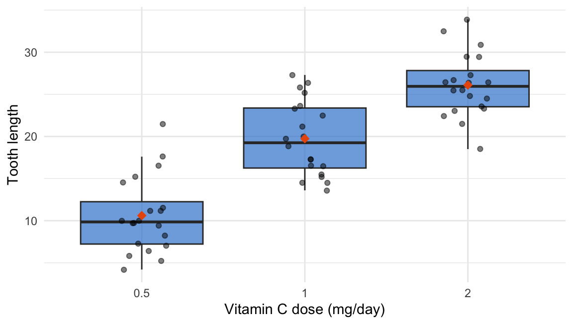
Drop that same p into a Word document:
doc <- read_docx()
doc <- body_add_par(doc, "Tooth growth by dose", style = "heading 2")
doc <- body_add_gg(doc, value = p, width = 6, height = 3.4)
print(doc, target = "chart-report.docx")
For an external image — a saved plot, a logo, a screenshot — use body_add_img() with a path and size:
ggsave("chart.png", p, width = 6, height = 3.4, dpi = 150)
doc <- body_add_img(doc, src = "chart.png", width = 6, height = 3.4)
body_add_gg() works with any grid-based graphic (ggplot2, lattice); body_add_img() accepts PNG, JPEG, and similar formats.
Page breaks and a table of contents
Long reports need structure. body_add_break() inserts a page break, and body_add_toc() drops in a table of contents that Word builds from your heading styles.
doc <- read_docx()

doc <- body_add_par(doc, "Report contents", style = "heading 1")
doc <- body_add_toc(doc)          # placeholder — Word fills it in
doc <- body_add_break(doc)        # start the body on a new page

doc <- body_add_par(doc, "Introduction", style = "heading 1")
doc <- body_add_par(doc, "Study background and objectives.", style = "Normal")
doc <- body_add_break(doc)

doc <- body_add_par(doc, "Results", style = "heading 1")
doc <- body_add_par(doc, "Findings and figures.", style = "Normal")

print(doc, target = "toc-report.docx")
Note
The TOC updates inside Word, not in R. body_add_toc() writes a field, not the finished list. The first time you open the file, Word asks to update fields — click Yes (or right-click the TOC → Update Field). Save afterwards so the entries stick.
Landscape pages for wide tables
A wide table or a broad chart often needs the page turned sideways. officer handles orientation per section: everything you add before a body_end_section_landscape() call becomes its own landscape section, and content after it continues in portrait.
doc <- read_docx()
doc <- body_add_par(doc, "Portrait intro", style = "heading 1")
doc <- body_add_par(doc, "This page stays portrait.", style = "Normal")

# The wide content that should sit sideways
doc <- body_add_par(doc, "A very wide table sits better sideways.", style = "Normal")
doc <- body_end_section_landscape(doc, w = 11, h = 8.5)   # close the landscape block

# Back to the default portrait orientation
doc <- body_add_par(doc, "Back to portrait for the discussion.", style = "Normal")

print(doc, target = "landscape-report.docx")
The w/h are the page width and height in inches (US Letter turned sideways here). For finer control — custom margins, columns, or an explicit portrait break — pass a full prop_section() to body_end_section_portrait() / body_end_section_continuous().
Start from a Word template
The real power move for a professional report: start from your own template — one with your logo, fonts, colours, and custom paragraph styles. Pass its path to read_docx() and every style it defines becomes available.
# Open your branded template instead of the blank default
doc <- read_docx(path = "corporate-template.docx")

# Discover the style names your template defines
styles_info(doc)

# Now use those styles by name
doc <- body_add_par(doc, "Quarterly Report", style = "Title")
doc <- body_add_par(doc, "Key point", style = "List Bullet")
Design the template once in Word (headers, footers, cover page, brand styles), then let R fill it with fresh numbers on every run — the report always looks on-brand without any manual formatting.
Put it together: a complete report
Here is the full pattern end to end — a title, an intro, a chart, and a summary table, written to a single .docx. This is the cover image of this post: a finished Word page, generated entirely from R.
library(officer)
library(flextable)
library(ggplot2)

# A chart
p <- ggplot(ToothGrowth, aes(factor(dose), len)) +
  geom_boxplot(fill = "#3a86d4", alpha = 0.7, outlier.shape = NA) +
  geom_jitter(width = 0.15, alpha = 0.5) +
  stat_summary(fun = mean, geom = "point", shape = 18, size = 3, color = "#e8590c") +
  labs(x = "Vitamin C dose (mg/day)", y = "Tooth length") +
  theme_minimal()

# A summary table: mean length per dose
tg <- aggregate(len ~ dose, data = ToothGrowth, FUN = mean)
names(tg) <- c("Dose (mg/day)", "Mean length")
ft <- autofit(theme_zebra(flextable(tg)))

# Assemble the document
doc <- read_docx()
doc <- body_add_par(doc, "Tooth growth report", style = "heading 1")
doc <- body_add_par(
  doc,
  "Guinea pig odontoblast length by vitamin C dose. Generated from R with officer.",
  style = "Normal"
)
doc <- body_add_par(doc, "Distribution by dose", style = "heading 2")
doc <- body_add_gg(doc, value = p, width = 6, height = 3.1)
doc <- body_add_par(doc, "Mean length by dose", style = "heading 2")
doc <- body_add_flextable(doc, ft)

print(doc, target = "report.docx")
Rerun the script after your data changes and the whole report — chart, table, numbers — rebuilds itself. That is the entire point: reports as code.
Frequently asked questions
NoteIs officer a replacement for ReporteRs?
Yes. ReporteRs was removed from CRAN and is no longer installable (it depended on Java and rJava). officer by the same author, David Gohel, is its modern, cross-platform, Java-free successor and the current community standard for generating Word and PowerPoint files from R. Every ReporteRs capability — titles, formatted text, tables, plots, page breaks, a table of contents — has an officer (plus flextable) equivalent, listed in the mapping table above.
NoteHow do I add bullet or numbered lists?
Use body_add_list() with a block_list_items() object — it writes the bullet or numbering definitions into the document itself, so no template is required (see Bulleted and numbered lists above). Set list_type = "bullet" or "decimal" and use level to nest. (The older body_add_par(doc, "item", style = "List Bullet") route still works, but only when your template already defines those paragraph styles — check with styles_info(doc).)
NoteWhat’s the difference between officer and officedown?
Use officer when you build a document programmatically in an R script — the block-by-block approach in this post. Use officedown when you author in R Markdown or Quarto and want the knitted Word output to gain officer features (captions, cross-references, landscape sections). officedown sits on top of officer; pick officer for scripted report generation, officedown for prose-first documents.
NoteCan officer also create PowerPoint slides?
Yes. read_pptx() opens a presentation and the add_slide() / ph_with() family places text, tables, and plots onto slide layouts — the same object-then-print pattern. One package covers both Word and PowerPoint reporting from R.
NoteDo I need Microsoft Word installed to generate the .docx?
No. officer writes the .docx file directly — it never launches Word, and it runs on Windows, macOS, and Linux (including headless servers and CI). You only need Word (or a compatible reader such as LibreOffice or Google Docs) to open the finished file.
Going deeper in /learn
This is the focused recipe for getting R output into Word. For the full, step-by-step lessons on building the charts you’ll embed:
- ggplot2 series — build the publication-ready figures that go straight into
body_add_gg(). - Data Visualization pillar — the complete visual toolkit, from boxplots to heatmaps.
Citation
BibTeX citation:
@online{kassambara2026,
  author = {Kassambara, Alboukadel},
  title = {Create {Word} {Documents} from {R} with Officer},
  date = {2026-07-08},
  url = {https://www.datanovia.com/blog/word-documents-in-r-officer},
  langid = {en}
}
For attribution, please cite this work as:
Kassambara, Alboukadel. 2026. “Create Word Documents from R with
Officer.” July 8. https://www.datanovia.com/blog/word-documents-in-r-officer.