ggiraph in Shiny: Click Selection and Reactivity in R
Read clicks from a girafe widget with opts_selection() and input$_selected — and save the chart to any report
Data Visualization
Drive a Shiny app from a chart with ggiraph — render a girafe widget with girafeOutput() and renderGirafe(), let readers click to select points with opts_selection(), read the selection reactively from input$<id>_selected for linked views and drilldown, and save or embed a girafe in any Quarto or R Markdown report.
Published
July 9, 2026
Modified
July 9, 2026
TipKey takeaways
Put a girafe chart in a Shiny app with girafeOutput("id") in the UI and renderGirafe({ girafe(...) }) in the server.
Add opts_selection() to girafe() so a click selects elements by their data_id — type = "single" or type = "multiple".
Read the selection reactively from input$<id>_selected — a character vector of the selected data_ids — to drive linked views, a detail table, or drilldown.
A girafe() object is a self-contained htmlwidget: it embeds in any Quarto/R Markdown HTML report and can be written to a standalone file with htmlwidgets::saveWidget().
ggiraph is free and open-source, and keeps ggplot2’s publication-grade look.
Introduction
You have a scatter plot in a dashboard and you want it to do something: the reader clicks a few points, and a table below fills in with their details — or a second chart redraws to show only what they picked. That click-to-select, linked-view pattern is the heart of an interactive dashboard, and ggiraph gives it to you without leaving ggplot2.
This lesson shows the Shiny side of ggiraph: how to render a girafe() widget in an app, how opts_selection() turns a click into a selection, and how to read that selection reactively in R to update the rest of the page. A live Shiny server can’t run inside this static lesson, so the app code is shown as plain R you can copy into app.R — but the selection itself works client-side, so the one live widget below lets you click and select right here. If you’re new to ggiraph, start with Getting started with ggiraph; here we assume you know the geom_*_interactive() + girafe() pattern.
The data
We use the built-in mtcars dataset — one row per car, with weight (wt), fuel efficiency (mpg), and horsepower (hp). Each car becomes one point, and the car name becomes the point’s data_id — the value a click will return.
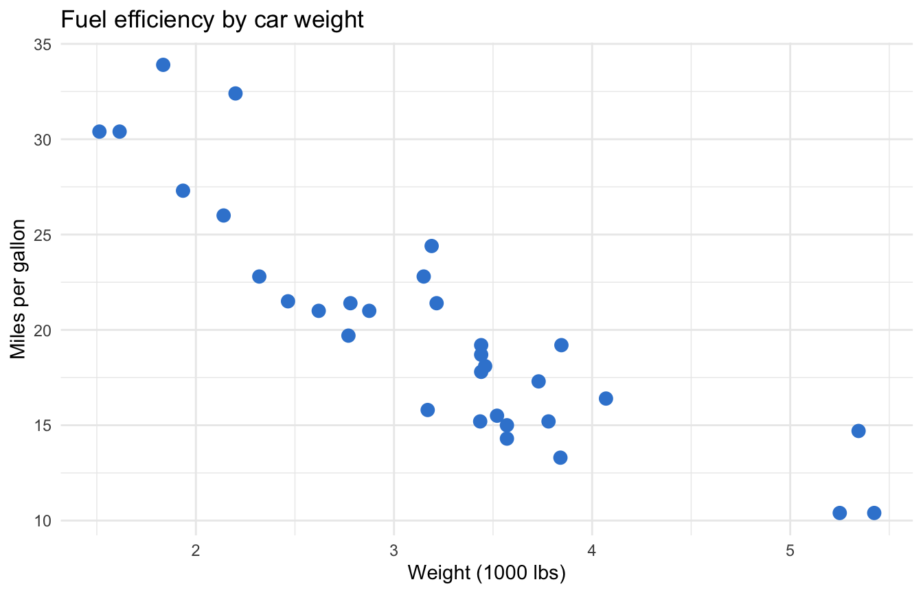
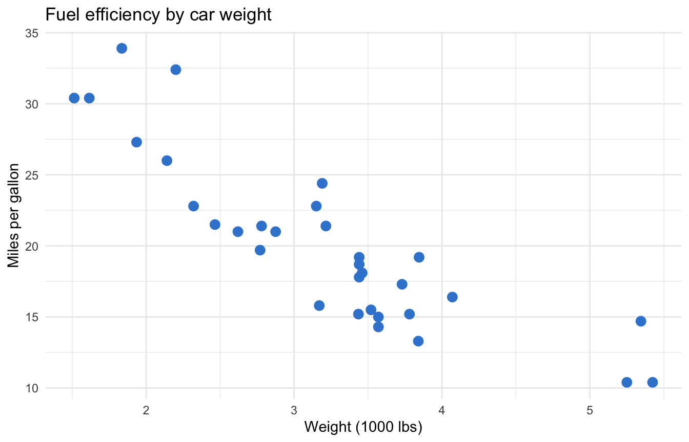
Here is the ordinary ggplot2 scatter plot — car weight against miles per gallon, brand-azure points, nothing interactive yet. This is the static figure the lesson builds on (and the chart you already know how to make).
library(ggplot2)ggplot(mtcars, aes(x = wt, y = mpg)) +geom_point(color ="#3a86d4", size =3) +labs(x ="Weight (1000 lbs)", y ="Miles per gallon",title ="Fuel efficiency by car weight") +theme_minimal()
To make it selectable, swap geom_point() for geom_point_interactive() and map two aesthetics: data_id (the value a click returns — the car name) and tooltip (what shows on hover). Everything else about the plot stays the same.
library(ggplot2)library(ggiraph)p <-ggplot(mtcars, aes(x = wt, y = mpg)) +geom_point_interactive(aes(data_id =rownames(mtcars), tooltip =rownames(mtcars)),color ="#3a86d4", size =3 ) +labs(x ="Weight (1000 lbs)", y ="Miles per gallon",title ="Fuel efficiency by car weight") +theme_minimal()p
Rendered as a static image, p looks identical to the first chart — the data_id and tooltip values are hidden metadata attached to each point. They come alive only when girafe() renders the plot as an interactive SVG.
Click to select: opts_selection()
opts_selection() is the option that makes elements selectable: click a point and it stays highlighted; click again to deselect. Its type argument controls how many things can be selected at once:
type
Behaviour
Selection returned
"single"
One element at a time; clicking another replaces it.
A length-1 character vector.
"multiple"
Click several; each toggles on/off.
A character vector of every selected data_id.
"none"
Selection off (the default).
—
The css argument styles the selected look — here a selected point turns amber (#f5a524) with a dark outline, so it stands out from both the azure default and the light-blue hover tint. One detail that trips everyone up outside Shiny:opts_selection() is Shiny-only by default, so on a static page (like this one, or a plain Quarto/R Markdown report) you must pass only_shiny = FALSE to turn click-selection on — without it, clicking does nothing. Set an explicit width_svg/height_svg so the widget reserves its space and the page doesn’t shift as it loads.
This widget is live — click any point (or several); each stays amber until you click it again. In a Shiny app the selected car names also arrive in R as input$<id>_selected, which the next section uses.
library(ggplot2)library(ggiraph)p <-ggplot(mtcars, aes(x = wt, y = mpg)) +geom_point_interactive(aes(data_id =rownames(mtcars), tooltip =rownames(mtcars)),color ="#3a86d4", size =3 ) +labs(x ="Weight (1000 lbs)", y ="Miles per gallon",title ="Click a point to select it") +theme_minimal()girafe(ggobj = p,width_svg =7,height_svg =4.5,options =list(# only_shiny = FALSE is essential OUTSIDE Shiny: by default opts_selection() is# Shiny-only, so clicks do nothing on a static page. Setting it FALSE enables# click-selection here. A selected point turns amber with a dark outline (it# persists); hovering only tints a point light blue (temporary).opts_selection(type ="multiple", only_shiny =FALSE,css ="fill:#f5a524;stroke:#0b2942;stroke-width:1.5pt;"),opts_hover(css ="fill:#8bb8e8;"),opts_tooltip(css ="background:#1b2b40;color:#ffffff;padding:5px 9px;border-radius:6px;font-family:sans-serif;font-size:13px;") ))
Selection is a client-side feature of the SVG, which is why it works in this static page. The reason it matters is that in Shiny that same selection is exposed to the server as a reactive value — so R can respond to it.
NoteShow the underlying data
An interactive SVG is opaque to screen readers, so here is the data behind the widget — the first rows of the cars plotted, with the data_id (the row name) each point carries.
First cars in mtcars; each point’s data_id is its row name (shown in the first column).
Weight (1000 lbs)
Miles per gallon
Horsepower
Mazda RX4
2.620
21.0
110
Mazda RX4 Wag
2.875
21.0
110
Datsun 710
2.320
22.8
93
Hornet 4 Drive
3.215
21.4
110
Hornet Sportabout
3.440
18.7
175
Valiant
3.460
18.1
105
Duster 360
3.570
14.3
245
Merc 240D
3.190
24.4
62
Put the widget in a Shiny app
Two functions bridge ggiraph and Shiny. In the UI, girafeOutput("plot") reserves a slot for the widget. In the server, renderGirafe({ girafe(...) }) builds it. The output id you pass to girafeOutput() — here "plot" — is what ties the widget to its selection input.
That app already works — you can click points and they highlight — but nothing reads the clicks yet. That’s the next step.
Read the selection reactively: input$<id>_selected
Here is the key rule: when a girafe output is named "plot" and its girafe() has opts_selection(), Shiny publishes the current selection as input$plot_selected — a character vector of the selected data_id values, updated reactively on every click. The pattern is always input$<outputId>_selected.
Because it’s a normal reactive input, you use it like any other: read it inside a render*() to build a linked view, or watch it with observeEvent(). This server adds a detail table that lists exactly the cars the reader selected:
server <-function(input, output) { output$plot <-renderGirafe({ p <-ggplot(mtcars, aes(x = wt, y = mpg)) +geom_point_interactive(aes(data_id =rownames(mtcars), tooltip =rownames(mtcars)),color ="#3a86d4", size =3 ) +theme_minimal()girafe(ggobj = p,options =list(opts_selection(type ="multiple", css ="fill:#f5a524;"))) })# Linked view: a table of the selected cars, redrawn on every click. output$picked <-renderTable({ selected <- input$plot_selected # character vector of selected data_idsif (length(selected) ==0) return(NULL) # nothing selected yet mtcars[selected, c("wt", "mpg", "hp")] # subset by the returned row names }, rownames =TRUE)}
Add tableOutput("picked") to the UI beneath girafeOutput("plot") and the table now tracks the selection live. The same input$plot_selected can drive anything reactive — filter a second chart, compute a summary of the chosen rows, or trigger a drilldown. To react to a click rather than render from it, wrap it in an observer:
With type = "single", input$plot_selected holds at most one value, so you can use it directly (for example mtcars[input$plot_selected, ]) for a classic click-one-row-see-its-detail drilldown.
Save or embed the girafe
A girafe() call returns an htmlwidget — the same object class as a leaflet map or a plotly chart — so it embeds and saves like any widget. Two things follow:
It embeds in any report automatically. Print a girafe() object in a Quarto document or an R Markdown HTML report and it renders inline, fully interactive, in the self-contained output file — no Shiny server required. That’s exactly what the live widget above is: a girafe printed in this Quarto page. Interactivity that needs a running server (the reactive input$plot_selected) only works inside Shiny; hover, tooltip, and click-selection highlighting work in any static HTML.
It writes to a standalone file. To hand someone a single self-contained HTML file of the chart, save the widget:
The resulting cars.html opens in any browser with tooltips and selection highlighting intact. This is the honest boundary to teach: the SVG interactivity travels with the file, but reading a selection in R is a Shiny-only capability because it needs the live reactive bridge.
🟢 With an AI agent
Ask Prova“how do I make a second ggiraph chart filter when I click a point in the first one?” — it answers with code you can run, so the explanation is reproducible. The runtime is the judge.Ask Prova →
Common issues
input$plot_selected is always NULL. The selection input only exists when the girafe() has opts_selection() in its options. Without it, clicks do nothing and no _selected input is published. Add opts_selection(type = "single") (or "multiple") and confirm the output id in input$<id>_selected matches the id you passed to girafeOutput() / output$<id>.
The selection returns the wrong values.input$plot_selected returns data_id values, not row numbers. Whatever you mapped to data_id is what comes back — so mtcars[input$plot_selected, ] works only because data_id = rownames(mtcars). If you map data_id to an index or a code, subset by that.
Nothing selects, but hover works. You likely used a non-interactive geom. Selection needs geom_*_interactive() (e.g. geom_point_interactive()) with a data_id aesthetic — a plain geom_point() has no ids to select.
Frequently asked questions
NoteHow do I display a ggiraph chart in a Shiny app?
Use the pair girafeOutput("id") in the UI and renderGirafe({ girafe(ggobj = p) }) in the server, where p is a ggplot built with geom_*_interactive(). The id you give girafeOutput() links the widget to its reactive inputs such as input$id_selected.
NoteHow do I get the clicked point from a ggiraph chart in Shiny?
Add opts_selection() to your girafe() call, then read input$<outputId>_selected in the server. It is a reactive character vector of the selected elements’ data_id values, updated on every click — use it inside a render*() for a linked view or in observeEvent() to react to the click.
NoteWhat is the difference between opts_selection type “single” and “multiple”?
type = "single" allows one selected element at a time — clicking another replaces it — so input$<id>_selected holds at most one value. type = "multiple" lets the reader toggle several elements on and off, and input$<id>_selected returns all of them. Use "single" for click-one-row drilldown and "multiple" for building up a set.
NoteCan I use a ggiraph chart without Shiny?
Yes. A girafe() object is a self-contained htmlwidget: printed in a Quarto or R Markdown HTML document it renders inline with tooltips, hover, and click-selection highlighting, and htmlwidgets::saveWidget() writes it to a standalone HTML file. Only reading a selection in R (input$<id>_selected) needs a running Shiny server.
NoteHow do I save a ggiraph chart as an HTML file?
Build the widget and pass it to htmlwidgets::saveWidget(), e.g. saveWidget(girafe(ggobj = p), "chart.html"). The output is a single self-contained file that opens in any browser with its interactivity intact.
Test your understanding
ImportantExercise: show the selected cars in a table
You have a Shiny app whose girafe output is named "plot" and whose girafe() uses opts_selection(type = "multiple"), with data_id = rownames(mtcars). Add a reactive table that lists the wt, mpg, and hp of exactly the cars the reader has selected, and shows nothing when the selection is empty.
TipHint
The selection arrives as input$plot_selected (pattern: input$<outputId>_selected) — a character vector of data_id values, which here are row names. Subset mtcars by it inside a renderTable(), and guard the empty case with if (length(...) == 0) return(NULL).
Because data_id = rownames(mtcars), input$plot_selected returns the selected row names, so mtcars[selected, ] pulls exactly those rows. The length(selected) == 0 guard shows nothing until the reader clicks. Add tableOutput("picked") to the UI to display it.
ImportantQuick check: what does input$plot_selected contain?
A girafe output named "plot" uses opts_selection() with data_id = rownames(mtcars). After the reader clicks two points, what is in input$plot_selected?
TipShow answer
A character vector of the two selected data_id values — here the two car names (row names), e.g. c("Mazda RX4", "Valiant"). It holds data_id values (not row numbers), which is why subsetting by it works only when data_id was mapped to the row names.
Conclusion
Two functions put a ggiraph chart in Shiny — girafeOutput() in the UI and renderGirafe() in the server — and opts_selection() turns clicks into a reactive selection you read from input$<id>_selected. From there it’s ordinary reactivity: drive a linked table, filter a second chart, or drilldown on a single click. And because a girafe is just an htmlwidget, the same chart drops into any Quarto or R Markdown report and saves to a standalone HTML file — you only need Shiny when you want R to read the selection.
This lesson is reproducible: the figures are executed at build time (if they render, the code works). Copy any block and run it to reproduce these charts. The runtime is the judge.
@online{2026,
  author = {},
  title = {Ggiraph in {Shiny:} {Click} {Selection} and {Reactivity} in
    {R}},
  date = {2026-07-09},
  url = {https://www.datanovia.com/learn/data-visualization/ggiraph/ggiraph-in-shiny},
  langid = {en}
}