Data Clustering Basics

Methods for measuring distances

The choice of distance measures is a critical step in clustering. It defines how the similarity of two elements (x, y) is calculated and it will influence the shape of the clusters.

The classical methods for distance measures are Euclidean and Manhattan distances, which are defined as follow:

1. Euclidean distance:

\[
d_{euc}(x,y) = \sqrt{\sum_{i=1}^n(x_i - y_i)^2}
\]

2. Manhattan distance:

\[
d_{man}(x,y) = \sum_{i=1}^n |{(x_i - y_i)|}
\]

Where, x and y are two vectors of length n.

Other dissimilarity measures exist such as correlation-based distances, which is widely used for gene expression data analyses. Correlation-based distance is defined by subtracting the correlation coefficient from 1. Different types of correlation methods can be used such as:

1. Pearson correlation distance:

\[
d_{cor}(x, y) = 1 - \frac{\sum\limits_{i=1}^n (x_i - \bar{x})(y_i - \bar{y})}{\sqrt{\sum\limits_{i=1}^n(x_i - \bar{x})^2 \sum\limits_{i=1}^n(y_i -\bar{y})^2}}
\]

2. Eisen cosine correlation distance (Eisen et al., 1998):

It’s a special case of Pearson’s correlation with \(\bar{x}\) and \(\bar{y}\) both replaced by zero:

\[
d_{eisen}(x, y) = 1 - \frac{\left|\sum\limits_{i=1}^n x_iy_i\right|}{\sqrt{\sum\limits_{i=1}^n x^2_i \sum\limits_{i=1}^n y^2_i}}
\]

3. Spearman correlation distance:

The spearman correlation method computes the correlation between the rank of x and the rank of y variables.

\[
d_{spear}(x, y) = 1 - \frac{\sum\limits_{i=1}^n (x'_i - \bar{x'})(y'_i - \bar{y'})}{\sqrt{\sum\limits_{i=1}^n(x'_i - \bar{x'})^2 \sum\limits_{i=1}^n(y'_i -\bar{y'})^2}}
\]

Where \(x'_i = rank(x_i)\) and \(y'_i = rank(y)\).

4. Kendall correlation distance:

Kendall correlation method measures the correspondence between the ranking of x and y variables. The total number of possible pairings of x with y observations is \(n(n-1)/2\), where n is the size of x and y. Begin by ordering the pairs by the x values. If x and y are correlated, then they would have the same relative rank orders. Now, for each \(y_i\), count the number of \(y_j > y_i\) (concordant pairs (c)) and the number of \(y_j < y_i\) (discordant pairs (d)).

Kendall correlation distance is defined as follow:

\[
d_{kend}(x, y) = 1 - \frac{n_c - n_d}{\frac{1}{2}n(n-1)}
\]

Where,

• \(n_c\): total number of concordant pairs
• \(n_d\): total number of discordant pairs
• \(n\): size of x and y

What type of distance measures should we choose?

The choice of distance measures is very important, as it has a strong influence on the clustering results. For most common clustering software, the default distance measure is the Euclidean distance.

Depending on the type of the data and the researcher questions, other dissimilarity measures might be preferred. For example, correlation-based distance is often used in gene expression data analysis.

Correlation-based distance considers two objects to be similar if their features are highly correlated, even though the observed values may be far apart in terms of Euclidean distance. The distance between two objects is 0 when they are perfectly correlated. Pearson’s correlation is quite sensitive to outliers. This does not matter when clustering samples, because the correlation is over thousands of genes. When clustering genes, it is important to be aware of the possible impact of outliers. This can be mitigated by using Spearman’s correlation instead of Pearson’s correlation.

If we want to identify clusters of observations with the same overall profiles regardless of their magnitudes, then we should go with correlation-based distance as a dissimilarity measure. This is particularly the case in gene expression data analysis, where we might want to consider genes similar when they are “up” and “down” together. It is also the case, in marketing if we want to identify group of shoppers with the same preference in term of items, regardless of the volume of items they bought.

If Euclidean distance is chosen, then observations with high values of features will be clustered together. The same holds true for observations with low values of features.

Data standardization

The value of distance measures is intimately related to the scale on which measurements are made. Therefore, variables are often scaled (i.e. standardized) before measuring the inter-observation dissimilarities. This is particularly recommended when variables are measured in different scales (e.g: kilograms, kilometers, centimeters, …); otherwise, the dissimilarity measures obtained will be severely affected.

The goal is to make the variables comparable. Generally variables are scaled to have i) standard deviation one and ii) mean zero.

The standardization of data is an approach widely used in the context of gene expression data analysis before clustering. We might also want to scale the data when the mean and/or the standard deviation of variables are largely different.

When scaling variables, the data can be transformed as follow:

\[
\frac{x_i - center(x)}{scale(x)}
\]

Where \(center(x)\) can be the mean or the median of x values, and \(scale(x)\) can be the standard deviation (SD), the interquartile range, or the MAD (median absolute deviation).

The R base function scale() can be used to standardize the data. It takes a numeric matrix as an input and performs the scaling on the columns.

Distance matrix computation

# Subset of the data
set.seed(123)
ss <- sample(1:50, 15)   # Take 15 random rows
df <- USArrests[ss, ]    # Subset the 15 rows
df.scaled <- scale(df)   # Standardize the variables

dist.eucl <- dist(df.scaled, method = "euclidean")

# Reformat as a matrix
# Subset the first 3 columns and rows and Round the values
round(as.matrix(dist.eucl)[1:3, 1:3], 1)

##              Iowa Rhode Island Maryland
## Iowa          0.0          2.8      4.1
## Rhode Island  2.8          0.0      3.6
## Maryland      4.1          3.6      0.0

# Compute
library("factoextra")
dist.cor <- get_dist(df.scaled, method = "pearson")

# Display a subset
round(as.matrix(dist.cor)[1:3, 1:3], 1)

##              Iowa Rhode Island Maryland
## Iowa          0.0          0.4      1.9
## Rhode Island  0.4          0.0      1.5
## Maryland      1.9          1.5      0.0

library(cluster)
# Load data
data(flower)
head(flower, 3)

##   V1 V2 V3 V4 V5 V6  V7 V8
## 1  0  1  1  4  3 15  25 15
## 2  1  0  0  2  1  3 150 50
## 3  0  1  0  3  3  1 150 50

# Data structure
str(flower)

## 'data.frame':    18 obs. of  8 variables:
##  $ V1: Factor w/ 2 levels "0","1": 1 2 1 1 1 1 1 1 2 2 ...
##  $ V2: Factor w/ 2 levels "0","1": 2 1 2 1 2 2 1 1 2 2 ...
##  $ V3: Factor w/ 2 levels "0","1": 2 1 1 2 1 1 1 2 1 1 ...
##  $ V4: Factor w/ 5 levels "1","2","3","4",..: 4 2 3 4 5 4 4 2 3 5 ...
##  $ V5: Ord.factor w/ 3 levels "1"<"2"<"3": 3 1 3 2 2 3 3 2 1 2 ...
##  $ V6: Ord.factor w/ 18 levels "1"<"2"<"3"<"4"<..: 15 3 1 16 2 12 13 7 4 14 ...
##  $ V7: num  25 150 150 125 20 50 40 100 25 100 ...
##  $ V8: num  15 50 50 50 15 40 20 15 15 60 ...

# Distance matrix
dd <- daisy(flower)
round(as.matrix(dd)[1:3, 1:3], 2)

##      1    2    3
## 1 0.00 0.89 0.53
## 2 0.89 0.00 0.51
## 3 0.53 0.51 0.00

Visualizing distance matrices

A simple solution for visualizing the distance matrices is to use the function fviz_dist() [factoextra package]. Other specialized methods, such as agglomerative hierarchical clustering or heatmap will be comprehensively described in the dedicated courses.

To use fviz_dist() type this:

library(factoextra)
fviz_dist(dist.eucl)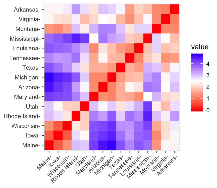

• Red: high similarity (ie: low dissimilarity) | Blue: low similarity

The color level is proportional to the value of the dissimilarity between observations: pure red if \(dist(x_i, x_j) = 0\) and pure blue corresponds to the highest value of euclidean distance computed. Objects belonging to the same cluster are displayed in consecutive order.

Summary

We described how to compute distance matrices using either Euclidean or correlation-based measures. It’s generally recommended to standardize the variables before distance matrix computation. Standardization makes variable comparable, in the situation where they are measured in different scales.