This article describes how to compare cluster dendrograms in R using the dendextend R package.
The dendextend package provides several functions for comparing dendrograms. Here, we’ll focus on two functions:
- tanglegram() for visual comparison of two dendrograms
- and cor.dendlist() for computing a correlation matrix between dendrograms.
Related Book
Practical Guide to Cluster Analysis in RData preparation
We’ll use the R base USArrests data sets and we start by standardizing the variables using the function scale() as follow:
df <- scale(USArrests)To make readable the plots, generated in the next sections, we’ll work with a small random subset of the data set. Therefore, we’ll use the function sample() to randomly select 10 observations among the 50 observations contained in the data set:
# Subset containing 10 rows
set.seed(123)
ss <- sample(1:50, 10)
df <- df[ss,]
Dendrograms comparison
We start by creating a list of two dendrograms by computing hierarchical clustering (HC) using two different linkage methods (“average” and “ward.D2”). Next, we transform the results as dendrograms and create a list to hold the two dendrograms.
library(dendextend)

# Compute distance matrix
res.dist <- dist(df, method = "euclidean")

# Compute 2 hierarchical clusterings
hc1 <- hclust(res.dist, method = "average")
hc2 <- hclust(res.dist, method = "ward.D2")

# Create two dendrograms
dend1 <- as.dendrogram (hc1)
dend2 <- as.dendrogram (hc2)

# Create a list to hold dendrograms
dend_list <- dendlist(dend1, dend2)- Visual comparison of two dendrograms
To visually compare two dendrograms, we’ll use the following R functions [dendextend package]:
- untangle(): finds the best layout to align dendrogram lists, using heuristic methods
- tanglegram(): plots the two dendrograms, side by side, with their labels connected by lines.
- entanglement(): computes the quality of the alignment of the two trees. Entanglement is a measure between 1 (full entanglement) and 0 (no entanglement). A lower entanglement coefficient corresponds to a good alignment.
- Draw a tanglegram:
# Align and plot two dendrograms side by side
dendlist(dend1, dend2) %>%
  untangle(method = "step1side") %>% # Find the best alignment layout
  tanglegram()                       # Draw the two dendrograms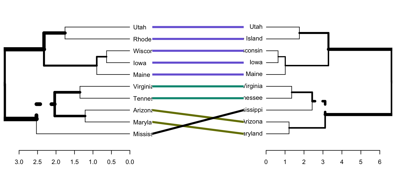
# Compute alignment quality. Lower value = good alignment quality
dendlist(dend1, dend2) %>%
  untangle(method = "step1side") %>% # Find the best alignment layout
  entanglement()                     # Alignment quality
## [1] 0.0384- Customized the tanglegram using many other options as follow:
dendlist(dend1, dend2) %>%
  untangle(method = "step1side") %>%
  tanglegram(
    highlight_distinct_edges = FALSE, # Turn-off dashed lines
    common_subtrees_color_lines = FALSE, # Turn-off line colors
    common_subtrees_color_branches = TRUE # Color common branches
    )
Note that, “unique” nodes, with a combination of labels/items not present in the other tree, are highlighted with dashed lines.
Note that, just because we can get two trees to have horizontal connecting lines, it doesn’t mean these trees are identical (or even very similar topologically).
In the following section, we’ll perform correlation analysis to measure the similarity between dendrograms.
- Correlation matrix between a list of dendrogams
The function cor.dendlist() is used to compute “Baker” or “Cophenetic” correlation matrix between a list of trees. The value can range between -1 to 1. With near 0 values meaning that the two trees are not statistically similar.
# Cophenetic correlation matrix
cor.dendlist(dend_list, method = "cophenetic")
## [,1] [,2]
## [1,] 1.000 0.965
## [2,] 0.965 1.000# Baker correlation matrix
cor.dendlist(dend_list, method = "baker")## [,1] [,2]
## [1,] 1.000 0.962
## [2,] 0.962 1.000The correlation between two trees can be also computed as follow:
# Cophenetic correlation coefficient
cor_cophenetic(dend1, dend2)
## [1] 0.965# Baker correlation coefficient
cor_bakers_gamma(dend1, dend2)## [1] 0.962It’s also possible to compare simultaneously multiple dendrograms. A chaining operator %>% is used to run multiple function at the same time. It’s useful for simplifying the code:
# Create multiple dendrograms by chaining
dend1 <- df %>% dist %>% hclust("complete") %>% as.dendrogram
dend2 <- df %>% dist %>% hclust("single") %>% as.dendrogram
dend3 <- df %>% dist %>% hclust("average") %>% as.dendrogram
dend4 <- df %>% dist %>% hclust("centroid") %>% as.dendrogram
# Compute correlation matrix
dend_list <- dendlist("Complete" = dend1, "Single" = dend2,
                      "Average" = dend3, "Centroid" = dend4)
cors <- cor.dendlist(dend_list)
# Print correlation matrix
round(cors, 2)
## Complete Single Average Centroid
## Complete 1.00 0.76 0.99 0.75
## Single 0.76 1.00 0.80 0.84
## Average 0.99 0.80 1.00 0.74
## Centroid 0.75 0.84 0.74 1.00# Visualize the correlation matrix using corrplot package
library(corrplot)
corrplot(cors, "pie", "lower")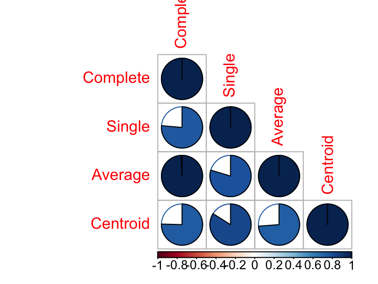
Recommended for you
This section contains best data science and self-development resources to help you on your path.
Books - Data Science
Our Books
- Practical Guide to Cluster Analysis in R by A. Kassambara (Datanovia)
- Practical Guide To Principal Component Methods in R by A. Kassambara (Datanovia)
- Machine Learning Essentials: Practical Guide in R by A. Kassambara (Datanovia)
- R Graphics Essentials for Great Data Visualization by A. Kassambara (Datanovia)
- GGPlot2 Essentials for Great Data Visualization in R by A. Kassambara (Datanovia)
- Network Analysis and Visualization in R by A. Kassambara (Datanovia)
- Practical Statistics in R for Comparing Groups: Numerical Variables by A. Kassambara (Datanovia)
- Inter-Rater Reliability Essentials: Practical Guide in R by A. Kassambara (Datanovia)
Others
- R for Data Science: Import, Tidy, Transform, Visualize, and Model Data by Hadley Wickham & Garrett Grolemund
- Hands-On Machine Learning with Scikit-Learn, Keras, and TensorFlow: Concepts, Tools, and Techniques to Build Intelligent Systems by Aurelien Géron
- Practical Statistics for Data Scientists: 50 Essential Concepts by Peter Bruce & Andrew Bruce
- Hands-On Programming with R: Write Your Own Functions And Simulations by Garrett Grolemund & Hadley Wickham
- An Introduction to Statistical Learning: with Applications in R by Gareth James et al.
- Deep Learning with R by François Chollet & J.J. Allaire
- Deep Learning with Python by François Chollet

No Comments