Many of the statistical methods including correlation, regression, t tests, and analysis of variance assume that the data follows a normal distribution or a Gaussian distribution. These tests are called parametric tests, because their validity depends on the distribution of the data.
Normality and the other assumptions made by these tests should be taken seriously to draw reliable interpretation and conclusions of the research.
With large enough sample sizes (> 30 or 40), there’s a pretty good chance that the data will be normally distributed; or at least close enough to normal that you can get away with using parametric tests, such as t-test (central limit theorem).
In this chapter, you will learn how to check the normality of the data in R by visual inspection (QQ plots and density distributions) and by significance tests (Shapiro-Wilk test).
Contents:
Related Book
Practical Statistics in R II - Comparing Groups: Numerical VariablesPrerequisites
Make sure you have installed the following R packages:
tidyversefor data manipulation and visualizationggpubrfor creating easily publication ready plotsrstatixprovides pipe-friendly R functions for easy statistical analyses
Start by loading the packages:
library(tidyverse)
library(ggpubr)
library(rstatix)
Demo data
We’ll use the ToothGrowth dataset. Inspect the data by displaying some random rows by groups:
set.seed(1234)
ToothGrowth %>% sample_n_by(supp, dose, size = 1)
## # A tibble: 6 x 3
## len supp dose
## <dbl> <fct> <dbl>
## 1 21.5 OJ 0.5
## 2 25.8 OJ 1
## 3 26.4 OJ 2
## 4 11.2 VC 0.5
## 5 18.8 VC 1
## 6 26.7 VC 2Examples of distribution shapes
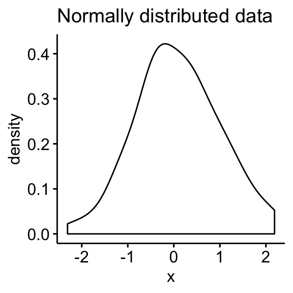
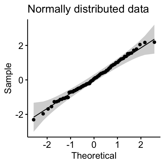
- Normal distribution
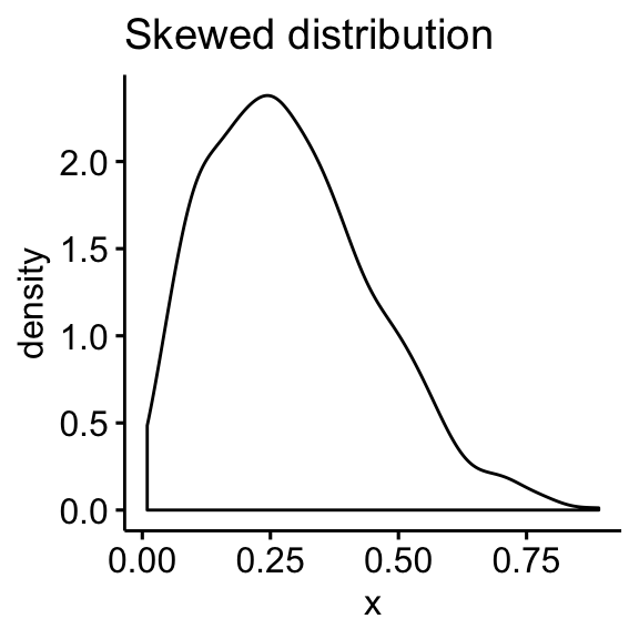
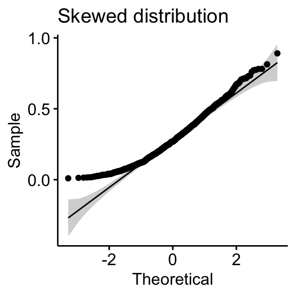
- Skewed distributions
Check normality in R
Question: We want to test if the variable len (tooth length) is normally distributed.
Visual methods
Density plot and Q-Q plot can be used to check normality visually.
- Density plot: the density plot provides a visual judgment about whether the distribution is bell shaped.
- QQ plot: QQ plot (or quantile-quantile plot) draws the correlation between a given sample and the normal distribution. A 45-degree reference line is also plotted. In a QQ plot, each observation is plotted as a single dot. If the data are normal, the dots should form a straight line.
library("ggpubr")
# Density plot
ggdensity(ToothGrowth$len, fill = "lightgray")
# QQ plot
ggqqplot(ToothGrowth$len)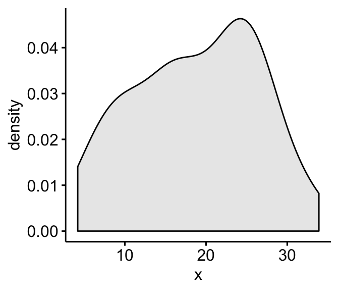
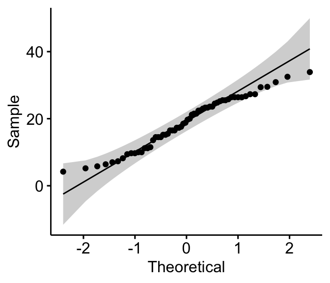
As all the points fall approximately along this reference line, we can assume normality.
Shapiro-Wilk’s normality test
Visual inspection, described in the previous section, is usually unreliable. It’s possible to use a significance test comparing the sample distribution to a normal one in order to ascertain whether data show or not a serious deviation from normality.
There are several methods for evaluate normality, including the Kolmogorov-Smirnov (K-S) normality test and the Shapiro-Wilk’s test.
The null hypothesis of these tests is that “sample distribution is normal”. If the test is significant, the distribution is non-normal.
Shapiro-Wilk’s method is widely recommended for normality test and it provides better power than K-S. It is based on the correlation between the data and the corresponding normal scores (Ghasemi and Zahediasl 2012).
Note that, normality test is sensitive to sample size. Small samples most often pass normality tests. Therefore, it’s important to combine visual inspection and significance test in order to take the right decision.
The R function shapiro_test() [rstatix package] provides a pipe-friendly framework to compute Shapiro-Wilk test for one or multiple variables. It also supports a grouped data. It’s a wrapper around R base function shapiro.test().
- Shapiro test for one variable:
ToothGrowth %>% shapiro_test(len)## # A tibble: 1 x 3
## variable statistic p
## <chr> <dbl> <dbl>
## 1 len 0.967 0.109From the output above, the p-value > 0.05 implying that the distribution of the data are not significantly different from normal distribution. In other words, we can assume the normality.
- Shapiro test for grouped data:
ToothGrowth %>%
  group_by(dose) %>%
  shapiro_test(len)
## # A tibble: 3 x 4
## dose variable statistic p
## <dbl> <chr> <dbl> <dbl>
## 1 0.5 len 0.941 0.247
## 2 1 len 0.931 0.164
## 3 2 len 0.978 0.902- Shapiro test for multiple variables:
iris %>% shapiro_test(Sepal.Length, Petal.Width)## # A tibble: 2 x 3
## variable statistic p
## <chr> <dbl> <dbl>
## 1 Petal.Width 0.902 0.0000000168
## 2 Sepal.Length 0.976 0.0102Summary
This chapter describes how to check the normality of a data using QQ-plot and Shapiro-Wilk test.
Note that, if your sample size is greater than 50, the normal QQ plot is preferred because at larger sample sizes the Shapiro-Wilk test becomes very sensitive even to a minor deviation from normality.
Consequently, we should not rely on only one approach for assessing the normality. A better strategy is to combine visual inspection and statistical test.
References
Ghasemi, Asghar, and Saleh Zahediasl. 2012. “Normality Tests for Statistical Analysis: A Guide for Non-Statisticians.” Int J Endocrinol Metab 10 (2): 486–89. doi:10.5812/ijem.3505.
Recommended for you
This section contains best data science and self-development resources to help you on your path.
Books - Data Science
Our Books
- Practical Guide to Cluster Analysis in R by A. Kassambara (Datanovia)
- Practical Guide To Principal Component Methods in R by A. Kassambara (Datanovia)
- Machine Learning Essentials: Practical Guide in R by A. Kassambara (Datanovia)
- R Graphics Essentials for Great Data Visualization by A. Kassambara (Datanovia)
- GGPlot2 Essentials for Great Data Visualization in R by A. Kassambara (Datanovia)
- Network Analysis and Visualization in R by A. Kassambara (Datanovia)
- Practical Statistics in R for Comparing Groups: Numerical Variables by A. Kassambara (Datanovia)
- Inter-Rater Reliability Essentials: Practical Guide in R by A. Kassambara (Datanovia)
Others
- R for Data Science: Import, Tidy, Transform, Visualize, and Model Data by Hadley Wickham & Garrett Grolemund
- Hands-On Machine Learning with Scikit-Learn, Keras, and TensorFlow: Concepts, Tools, and Techniques to Build Intelligent Systems by Aurelien Géron
- Practical Statistics for Data Scientists: 50 Essential Concepts by Peter Bruce & Andrew Bruce
- Hands-On Programming with R: Write Your Own Functions And Simulations by Garrett Grolemund & Hadley Wickham
- An Introduction to Statistical Learning: with Applications in R by Gareth James et al.
- Deep Learning with R by François Chollet & J.J. Allaire
- Deep Learning with Python by François Chollet
Version:
 Français

can you please give a reference to the book or paper that support the claims you do in this lesson: eg. “Note that, normality test is sensitive to sample size. Small samples most often pass normality tests. Therefore, it’s important to combine visual inspection and significance test in order to take the right decision.”