Statistical Tests and Assumptions

Non-normal distributions

Skewness is a measure of symmetry for a distribution. The value can be positive, negative or undefined. In a skewed distribution, the central tendency measures (mean, median, mode) will not be equal.

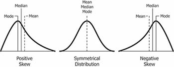
(Image courtesy: https://www.safaribooksonline.com/library/view/clojure-for-data/9781784397180/ch01s13.html)

• Positively skewed distribution (or right skewed): The most frequent values are low; tail is toward the high values (on the right-hand side). Generally, Mode < Median < Mean.
• Negatively skewed distribution (or left skewed), the most frequent values are high; tail is toward low values (on the left-hand side). Generally, Mode > Median > Mean.

The direction of skewness is given by the sign of the skewness coefficient:

• A zero means no skewness at all (normal distribution).
• A negative value means the distribution is negatively skewed.
• A positive value means the distribution is positively skewed.

The skewness coefficient can be computed using the moments R packages:

library(moments)
skewness(iris$Sepal.Length, na.rm = TRUE)

## [1] 0.312

Transformation methods

This section describes different transformation methods, depending to the type of normality violation.

Some common heuristics transformations for non-normal data include:

• square-root for moderate skew:
  • sqrt(x) for positively skewed data,
  • sqrt(max(x+1) - x) for negatively skewed data
• log for greater skew:
  • log10(x) for positively skewed data,
  • log10(max(x+1) - x) for negatively skewed data
• inverse for severe skew:
  • 1/x for positively skewed data
  • 1/(max(x+1) - x) for negatively skewed data
• Linearity and heteroscedasticity:
  • first try log transformation in a situation where the dependent variable starts to increase more rapidly with increasing independent variable values
  • If your data does the opposite – dependent variable values decrease more rapidly with increasing independent variable values – you can first consider a square transformation.

Examples of transforming skewed data

library(ggpubr)
library(moments)

data("USJudgeRatings")
df <- USJudgeRatings
head(df)

##                CONT INTG DMNR DILG CFMG DECI PREP FAMI ORAL WRIT PHYS RTEN
## AARONSON,L.H.   5.7  7.9  7.7  7.3  7.1  7.4  7.1  7.1  7.1  7.0  8.3  7.8
## ALEXANDER,J.M.  6.8  8.9  8.8  8.5  7.8  8.1  8.0  8.0  7.8  7.9  8.5  8.7
## ARMENTANO,A.J.  7.2  8.1  7.8  7.8  7.5  7.6  7.5  7.5  7.3  7.4  7.9  7.8
## BERDON,R.I.     6.8  8.8  8.5  8.8  8.3  8.5  8.7  8.7  8.4  8.5  8.8  8.7
## BRACKEN,J.J.    7.3  6.4  4.3  6.5  6.0  6.2  5.7  5.7  5.1  5.3  5.5  4.8
## BURNS,E.B.      6.2  8.8  8.7  8.5  7.9  8.0  8.1  8.0  8.0  8.0  8.6  8.6

# Distribution of CONT variable
ggdensity(df, x = "CONT", fill = "lightgray", title = "CONT") +
  scale_x_continuous(limits = c(3, 12)) +
  stat_overlay_normal_density(color = "red", linetype = "dashed")

# Distribution of PHYS variable
ggdensity(df, x = "PHYS", fill = "lightgray", title = "PHYS") +
  scale_x_continuous(limits = c(3, 12)) +
  stat_overlay_normal_density(color = "red", linetype = "dashed")

skewness(df$CONT, na.rm = TRUE)

## [1] 1.09

skewness(df$PHYS, na.rm = TRUE)

## [1] -1.56

df$CONT <- log10(df$CONT)
df$PHYS <- log10(max(df$CONT+1) - df$CONT)

# Distribution of CONT variable
ggdensity(df, x = "CONT", fill = "lightgray", title = "CONT") +
  stat_overlay_normal_density(color = "red", linetype = "dashed")

# Distribution of PHYS variable
ggdensity(df, x = "PHYS", fill = "lightgray", title = "PHYS") +
  stat_overlay_normal_density(color = "red", linetype = "dashed")

skewness(df$CONT, na.rm = TRUE)

## [1] 0.656

skewness(df$PHYS, na.rm = TRUE)

## [1] -0.818

Summary and discussion

This article describes how to transform data for normality, an assumption required for parametric tests such as t-tests and ANOVA tests.

In the situation where the normality assumption is not met, you could consider running the statistical tests (t-test or ANOVA) on the transformed and non-transformed data to see if there are any meaningful differences.

If both tests lead you to the same conclusions, you might not choose to transform the outcome variable and carry on with the test outputs on the original data.

Note that transformation makes the interpretation of the analysis much more difficult. For example, if you run a t-test for comparing the mean of two groups after transforming the data, you cannot simply say that there is a difference in the two groups’ means. Now, you have the added step of interpreting the fact that the difference is based on the log transformation. For this reason, transformations are usually avoided unless necessary for the analysis to be valid.

For analyses like the F or t family of tests (i.e., independent and dependent sample t-tests, ANOVAs, MANOVAs, and regressions), violations of normality are not usually a death sentence for validity. With large enough sample sizes (> 30 or 40), there’s a pretty good chance that the data will be normally distributed; or at least close enough to normal that you can get away with using parametric tests (central limit theorem).