The t-test is used to compare two means.
This chapter describes the different types of t-test, including:
- one-sample t-tests,
- independent samples t-tests: Student’s t-test and Welch’s t-test
- paired samples t-test.
You will learn how to:
- Compute the different t-tests in R. The pipe-friendly function
t_test()[rstatix package] will be used. - Check t-test assumptions
- Calculate and report t-test effect size using Cohen’s d. The
dstatistic redefines the difference in means as the number of standard deviations that separates those means. T-test conventional effect sizes, proposed by Cohen, are: 0.2 (small effect), 0.5 (moderate effect) and 0.8 (large effect) (Cohen 1998).
Contents:
Related Book
Practical Statistics in R II - Comparing Groups: Numerical VariablesPrerequisites
Make sure you have installed the following R packages:
tidyversefor data manipulation and visualizationggpubrfor creating easily publication ready plotsrstatixprovides pipe-friendly R functions for easy statistical analyses.datarium: contains required data sets for this chapter.
Start by loading the following required packages:
library(tidyverse)
library(ggpubr)
library(rstatix)
One-Sample t-test
The one-sample t-test, also known as the single-parameter t test or single-sample t-test, is used to compare the mean of one sample to a known standard (or theoretical / hypothetical) mean.
Generally, the theoretical mean comes from:
- a previous experiment. For example, comparing whether the mean weight of mice differs from 200 mg, a value determined in a previous study.
- or from an experiment where you have control and treatment conditions. If you express your data as “percent of control”, you can test whether the average value of treatment condition differs significantly from 100.
Demo data
Demo dataset: mice [in datarium package]. Contains the weight of 10 mice:
# Load and inspect the data
data(mice, package = "datarium")
head(mice, 3)
## # A tibble: 3 x 2
## name weight
## <chr> <dbl>
## 1 M_1 18.9
## 2 M_2 19.5
## 3 M_3 23.1Summary statistics
Compute some summary statistics: count (number of subjects), mean and sd (standard deviation)
mice %>% get_summary_stats(weight, type = "mean_sd")## # A tibble: 1 x 4
## variable n mean sd
## <chr> <dbl> <dbl> <dbl>
## 1 weight 10 20.1 1.90Visualization
Create a boxplot to visualize the distribution of mice weights. Add also jittered points to show individual observations. The big dot represents the mean point.
bxp <- ggboxplot(
  mice$weight, width = 0.5, add = c("mean", "jitter"),
  ylab = "Weight (g)", xlab = FALSE
  )
bxp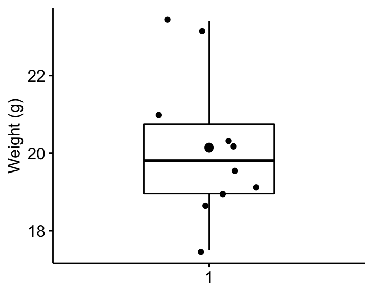
Assumptions and preliminary tests
The one-sample t-test assumes the following characteristics about the data:
- No significant outliers in the data
- Normality. the data should be approximately normally distributed
In this section, we’ll perform some preliminary tests to check whether these assumptions are met.
Identify outliers
Outliers can be easily identified using boxplot methods, implemented in the R function identify_outliers() [rstatix package].
mice %>% identify_outliers(weight)## # A tibble: 0 x 4
## # … with 4 variables: name <chr>, weight <dbl>, is.outlier <lgl>, is.extreme <lgl>There were no extreme outliers.
Note that, in the situation where you have extreme outliers, this can be due to: 1) data entry errors, measurement errors or unusual values.
In this case, you could consider running the non parametric Wilcoxon test.
Check normality assumption
The normality assumption can be checked by computing the Shapiro-Wilk test. If the data is normally distributed, the p-value should be greater than 0.05.
mice %>% shapiro_test(weight)## # A tibble: 1 x 3
## variable statistic p
## <chr> <dbl> <dbl>
## 1 weight 0.923 0.382From the output, the p-value is greater than the significance level 0.05 indicating that the distribution of the data are not significantly different from the normal distribution. In other words, we can assume the normality.
You can also create a QQ plot of the weight data. QQ plot draws the correlation between a given data and the normal distribution.
ggqqplot(mice, x = "weight")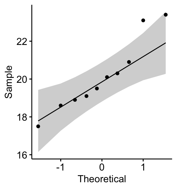
All the points fall approximately along the (45-degree) reference line, for each group. So we can assume normality of the data.
Note that, if your sample size is greater than 50, the normal QQ plot is preferred because at larger sample sizes the Shapiro-Wilk test becomes very sensitive even to a minor deviation from normality.
If the data are not normally distributed, it’s recommended to use a non-parametric test such as the one-sample Wilcoxon signed-rank test. This test is similar to the one-sample t-test, but focuses on the median rather than the mean.
Computation
We want to know, whether the average weight of the mice differs from the 25g (two-tailed test)?
stat.test <- mice %>% t_test(weight ~ 1, mu = 25)
stat.test
## # A tibble: 1 x 7
## .y. group1 group2 n statistic df p
## * <chr> <chr> <chr> <int> <dbl> <dbl> <dbl>
## 1 weight 1 null model 10 -8.10 9 0.00002The results above show the following components:
.y.: the outcome variable used in the test.group1,group2: generally, the compared groups in the pairwise tests. Here, we have null model (one-sample test).statistic: test statistic (t-value) used to compute the p-value.df: degrees of freedom.p: p-value.
You can obtain a detailed result by specifying the option detailed = TRUE in the function t_test().
Effect size
To calculate an effect size, called Cohen's d, for the one-sample t-test you need to divide the mean difference by the standard deviation of the difference, as shown below. Note that, here: sd(x-mu) = sd(x).
Cohen’s d formula:
d = abs(mean(x) - mu)/sd(x), where:
xis a numeric vector containing the data.muis the mean against which the mean of x is compared (default value is mu = 0).
Calculation:
mice %>% cohens_d(weight ~ 1, mu = 25)## # A tibble: 1 x 6
## .y. group1 group2 effsize n magnitude
## * <chr> <chr> <chr> <dbl> <int> <ord>
## 1 weight 1 null model 10.6 10 largeRecall that, t-test conventional effect sizes, proposed by Cohen J. (1998), are: 0.2 (small effect), 0.5 (moderate effect) and 0.8 (large effect) (Cohen 1998). As the effect size, d, is 2.56 you can conclude that there is a large effect.
Report
We could report the result as follow:
A one-sample t-test was computed to determine whether the recruited mice average weight was different to the population normal mean weight (25g).
The mice weight value were normally distributed, as assessed by Shapiro-Wilk’s test (p > 0.05) and there were no extreme outliers in the data, as assessed by boxplot method.
The measured mice mean weight (20.14 +/- 1.94) was statistically significantly lower than the population normal mean weight 25 (t(9) = -8.1, p < 0.0001, d = 2.56); where t(9) is shorthand notation for a t-statistic that has 9 degrees of freedom.
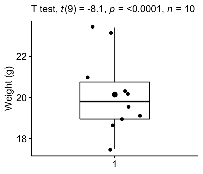
Create a box plot with p-value:
bxp + labs(
  subtitle = get_test_label(stat.test, detailed = TRUE)
  )
Create a density plot with p-value:
- Red line corresponds to the observed mean
- Blue line corresponds to the theoretical mean
ggdensity(mice, x = "weight", rug = TRUE, fill = "lightgray") +
  scale_x_continuous(limits = c(15, 27)) +
  stat_central_tendency(type = "mean", color = "red", linetype = "dashed") +
  geom_vline(xintercept = 25, color = "blue", linetype = "dashed") +
  labs(subtitle = get_test_label(stat.test,  detailed = TRUE))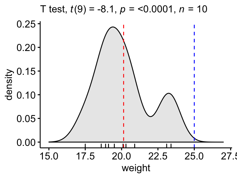
Independent samples t-test
The independent samples t-test (or unpaired samples t-test) is used to compare the mean of two independent groups.
For example, you might want to compare the average weights of individuals grouped by gender: male and female groups, which are two unrelated/independent groups.
The independent samples t-test comes in two different forms:
- the standard Student’s t-test, which assumes that the variance of the two groups are equal.
- the Welch’s t-test, which is less restrictive compared to the original Student’s test. This is the test where you do not assume that the variance is the same in the two groups, which results in the fractional degrees of freedom.
By default, R computes the Weltch t-test, which is the safer one. The two methods give very similar results unless both the group sizes and the standard deviations are very different.
Demo data
Demo dataset: genderweight [in datarium package] containing the weight of 40 individuals (20 women and 20 men).
Load the data and show some random rows by groups:
# Load the data
data("genderweight", package = "datarium")
# Show a sample of the data by group
set.seed(123)
genderweight %>% sample_n_by(group, size = 2)
## # A tibble: 4 x 3
## id group weight
## <fct> <fct> <dbl>
## 1 6 F 65.0
## 2 15 F 65.9
## 3 29 M 88.9
## 4 37 M 77.0Summary statistics
Compute some summary statistics by groups: mean and sd (standard deviation)
genderweight %>%
  group_by(group) %>%
  get_summary_stats(weight, type = "mean_sd")
## # A tibble: 2 x 5
## group variable n mean sd
## <fct> <chr> <dbl> <dbl> <dbl>
## 1 F weight 20 63.5 2.03
## 2 M weight 20 85.8 4.35Visualization
Visualize the data using box plots. Plot weight by groups.
bxp <- ggboxplot(
  genderweight, x = "group", y = "weight",
  ylab = "Weight", xlab = "Groups", add = "jitter"
  )
bxp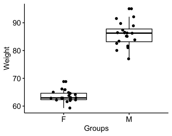
Assumptions and preliminary tests
The two-samples independent t-test assume the following characteristics about the data:
- Independence of the observations. Each subject should belong to only one group. There is no relationship between the observations in each group.
- No significant outliers in the two groups
- Normality. the data for each group should be approximately normally distributed.
- Homogeneity of variances. the variance of the outcome variable should be equal in each group.
In this section, we’ll perform some preliminary tests to check whether these assumptions are met.
Identify outliers by groups
genderweight %>%
  group_by(group) %>%
  identify_outliers(weight)
## # A tibble: 2 x 5
## group id weight is.outlier is.extreme
## <fct> <fct> <dbl> <lgl> <lgl>
## 1 F 20 68.8 TRUE FALSE
## 2 M 31 95.1 TRUE FALSEThere were no extreme outliers.
Check normality by groups
# Compute Shapiro wilk test by goups
data(genderweight, package = "datarium")
genderweight %>%
  group_by(group) %>%
  shapiro_test(weight)
## # A tibble: 2 x 4
## group variable statistic p
## <fct> <chr> <dbl> <dbl>
## 1 F weight 0.938 0.224
## 2 M weight 0.986 0.989# Draw a qq plot by group
ggqqplot(genderweight, x = "weight", facet.by = "group")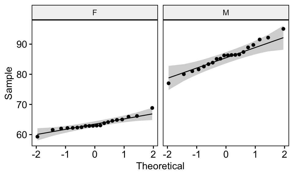
From the output above, we can conclude that the data of the two groups are normally distributed.
Check the equality of variances
This can be done using the Levene’s test. If the variances of groups are equal, the p-value should be greater than 0.05.
genderweight %>% levene_test(weight ~ group)## # A tibble: 1 x 4
## df1 df2 statistic p
## <int> <int> <dbl> <dbl>
## 1 1 38 6.12 0.0180The p-value of the Levene’s test is significant, suggesting that there is a significant difference between the variances of the two groups. Therefore, we’ll use the Weltch t-test, which doesn’t assume the equality of the two variances.
Computation
We want to know, whether the average weights are different between groups.
Recall that, by default, R computes the Weltch t-test, which is the safer one:
stat.test <- genderweight %>%
  t_test(weight ~ group) %>%
  add_significance()
stat.test
## # A tibble: 1 x 9
## .y. group1 group2 n1 n2 statistic df p p.signif
## <chr> <chr> <chr> <int> <int> <dbl> <dbl> <dbl> <chr>
## 1 weight F M 20 20 -20.8 26.9 4.30e-18 ****If you want to assume the equality of variances (Student t-test), specify the option var.equal = TRUE:
stat.test2 <- genderweight %>%
  t_test(weight ~ group, var.equal = TRUE) %>%
  add_significance()
stat.test2
The output is similar to the result of one-sample test. Recall that, more details can be obtained by specifying the option detailed = TRUE in the function t_test(). The p-value of the comparison is significant (p < 0.0001).
Effect size
Cohen’s d for Student t-test
This effect size is calculated by dividing the mean difference between the groups by the pooled standard deviation.
Cohen’s d formula:
d = (mean1 - mean2)/pooled.sd, where:
pooled.sdis the common standard deviation of the two groups.pooled.sd = sqrt([var1*(n1-1) + var2*(n2-1)]/[n1 + n2 -2]);var1andvar2are the variances (squared standard deviation) of group1 and 2, respectively.n1andn2are the sample counts for group 1 and 2, respectively.mean1andmean2are the means of each group, respectively.
Calculation:
genderweight %>% cohens_d(weight ~ group, var.equal = TRUE)## # A tibble: 1 x 7
## .y. group1 group2 effsize n1 n2 magnitude
## * <chr> <chr> <chr> <dbl> <int> <int> <ord>
## 1 weight F M 6.57 20 20 largeThere is a large effect size, d = 6.57.
Cohen’s d for Welch t-test
The Welch test is a variant of t-test used when the equality of variance can’t be assumed. The effect size can be computed by dividing the mean difference between the groups by the “averaged” standard deviation.
Cohen’s d formula:
d = (mean1 - mean2)/sqrt((var1 + var2)/2), where:
mean1andmean2are the means of each group, respectivelyvar1andvar2are the variance of the two groups.
Calculation:
genderweight %>% cohens_d(weight ~ group, var.equal = FALSE)## # A tibble: 1 x 7
## .y. group1 group2 effsize n1 n2 magnitude
## * <chr> <chr> <chr> <dbl> <int> <int> <ord>
## 1 weight F M 6.57 20 20 largeNote that, when group sizes are equal and group variances are homogeneous, Cohen’s d for the standard Student and Welch t-tests are identical.
Report
We could report the result as follow:
The mean weight in female group was 63.5 (SD = 2.03), whereas the mean in male group was 85.8 (SD = 4.3). A Welch two-samples t-test showed that the difference was statistically significant, t(26.9) = -20.8, p < 0.0001, d = 6.57; where, t(26.9) is shorthand notation for a Welch t-statistic that has 26.9 degrees of freedom.
stat.test <- stat.test %>% add_xy_position(x = "group")
bxp +
  stat_pvalue_manual(stat.test, tip.length = 0) +
  labs(subtitle = get_test_label(stat.test, detailed = TRUE))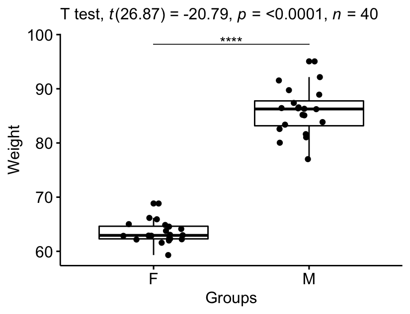
Paired samples t-test
The paired sample t-test is used to compare the means of two related groups of samples. Put into another words, it’s used in a situation where you have two pairs of values measured for the same samples.
For example, you might want to compare the average weight of 20 mice before and after treatment. The data contain 20 sets of values before treatment and 20 sets of values after treatment from measuring twice the weight of the same mice. In such situations, paired t-test can be used to compare the mean weights before and after treatment.
Demo data
Here, we’ll use a demo dataset mice2 [datarium package], which contains the weight of 10 mice before and after the treatment.
# Wide format
data("mice2", package = "datarium")
head(mice2, 3)
## id before after
## 1 1 187 430
## 2 2 194 404
## 3 3 232 406# Transform into long data:
# gather the before and after values in the same column
mice2.long <- mice2 %>%
gather(key = "group", value = "weight", before, after)
head(mice2.long, 3)## id group weight
## 1 1 before 187
## 2 2 before 194
## 3 3 before 232Summary statistics
Compute some summary statistics (mean and sd) by groups:
mice2.long %>%
  group_by(group) %>%
  get_summary_stats(weight, type = "mean_sd")
## # A tibble: 2 x 5
## group variable n mean sd
## <chr> <chr> <dbl> <dbl> <dbl>
## 1 after weight 10 400. 30.1
## 2 before weight 10 201. 20.0Visualization
bxp <- ggpaired(mice2.long, x = "group", y = "weight",
         order = c("before", "after"),
         ylab = "Weight", xlab = "Groups")
bxp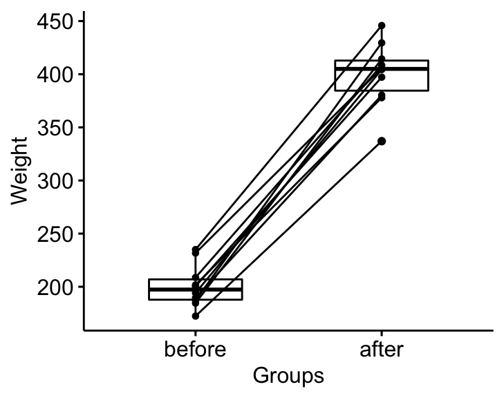
Assumptions and preliminary tests
The paired samples t-test assume the following characteristics about the data:
- the two groups are paired. In our example, this is the case since the data have been collected from measuring twice the weight of the same mice.
- No significant outliers in the difference between the two related groups
- Normality. the difference of pairs follow a normal distribution.
In this section, we’ll perform some preliminary tests to check whether these assumptions are met.
First, start by computing the difference between groups:
mice2 <- mice2 %>% mutate(differences = before - after)
head(mice2, 3)
## id before after differences
## 1 1 187 430 -242
## 2 2 194 404 -210
## 3 3 232 406 -174Identify outliers
mice2 %>% identify_outliers(differences)## [1] id before after differences is.outlier is.extreme
## <0 rows> (or 0-length row.names)There were no extreme outliers.
Check normality assumption
# Shapiro-Wilk normality test for the differences
mice2 %>% shapiro_test(differences)
## # A tibble: 1 x 3
## variable statistic p
## <chr> <dbl> <dbl>
## 1 differences 0.968 0.867# QQ plot for the difference
ggqqplot(mice2, "differences")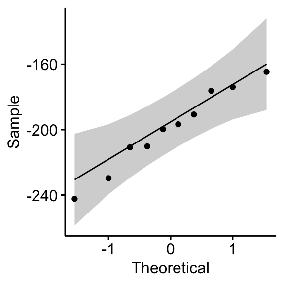
From the output above, it can be assumed that the differences are normally distributed.
Computation
We want to know, if there is any significant difference in the mean weights after treatment?
stat.test <- mice2.long  %>%
  t_test(weight ~ group, paired = TRUE) %>%
  add_significance()
stat.test
## # A tibble: 1 x 9
## .y. group1 group2 n1 n2 statistic df p p.signif
## <chr> <chr> <chr> <int> <int> <dbl> <dbl> <dbl> <chr>
## 1 weight after before 10 10 25.5 9 0.00000000104 ****The output is similar to that of a one-sample t-test. Again, more details can be obtained by specifying the option detailed = TRUE in the function t_test().
Effect size
The effect size for a paired-samples t-test can be calculated by dividing the mean difference by the standard deviation of the difference, as shown below.
Cohen’s formula:
d = mean(D)/sd(D), where D is the differences of the paired samples values.
Calculation:
mice2.long %>% cohens_d(weight ~ group, paired = TRUE)## # A tibble: 1 x 7
## .y. group1 group2 effsize n1 n2 magnitude
## * <chr> <chr> <chr> <dbl> <int> <int> <ord>
## 1 weight after before 8.08 10 10 largeThere is a large effect size, Cohen’s d = 8.07.
Report
We could report the result as follow: The average weight of mice was significantly increased after treatment, t(9) = 25.5, p < 0.0001, d = 8.07.
stat.test <- stat.test %>% add_xy_position(x = "group")
bxp +
  stat_pvalue_manual(stat.test, tip.length = 0) +
  labs(subtitle = get_test_label(stat.test, detailed= TRUE))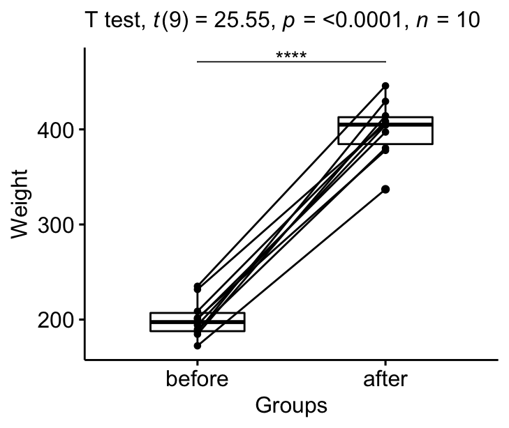
Summary
This chapter describes how to compare two means in R using t-test. Quick start R codes, to compute the different t-tests, are:
# One-sample t-test
mice %>% t_test(weight ~ 1, mu = 25)
# Independent samples t-test
genderweight %>% t_test(weight ~ group)
# Paired sample t-test
mice2.long %>% t_test(weight ~ group, paired = TRUE)
Note that, to compute one-sided t-tests, you can specify the option alternative, which possible values can be “greater”, “less” or “two.sided”.
We also explain the assumptions made by the t-test and provide practical examples of R codes to check whether the test assumptions are met.
The t-test assumptions can be summarized as follow:
- One-sample t-test:
- No significant outliers in the data
- the data should be normally distributed.
- Independent sample t-test:
- No significant outliers in the groups
- the two groups of samples (A and B), being compared, should be normally distributed.
- the variances of the two groups should not be significantly different. This assumption is made only by the original Student’s t-test. It is relaxed in the Welch’s t-test.
- Paired sample t-test:
- No significant outliers in the differences between groups
- the difference of pairs should follow a normal distribution.
Assessing normality. With large enough samples size (n > 30) the violation of the normality assumption should not cause major problems (according to the central limit theorem). This implies that we can ignore the distribution of the data and use parametric tests. However, to be consistent, the Shapiro-Wilk test can be used to ascertain whether data show or not a serious deviation from normality (See Chapter @ref(normality-test-in-r)).
Assessing equality of variances. Homogeneity of variances can be checked using the Levene’s test. Note that, by default, the t_test() function does not assume equal variances; instead of the standard Student’s t-test, it uses the Welch t-test by default, which is the considered the safer one. To use Student’s t-test, set var.equal = TRUE. The two methods give very similar results unless both the group sizes and the standard deviations are very different.
In the situations where the assumptions are violated, non-parametric tests, such as Wilcoxon test, are recommended.
References
Cohen, J. 1998. Statistical Power Analysis for the Behavioral Sciences. 2nd ed. Hillsdale, NJ: Lawrence Erlbaum Associates.
Recommended for you
This section contains best data science and self-development resources to help you on your path.
Books - Data Science
Our Books
- Practical Guide to Cluster Analysis in R by A. Kassambara (Datanovia)
- Practical Guide To Principal Component Methods in R by A. Kassambara (Datanovia)
- Machine Learning Essentials: Practical Guide in R by A. Kassambara (Datanovia)
- R Graphics Essentials for Great Data Visualization by A. Kassambara (Datanovia)
- GGPlot2 Essentials for Great Data Visualization in R by A. Kassambara (Datanovia)
- Network Analysis and Visualization in R by A. Kassambara (Datanovia)
- Practical Statistics in R for Comparing Groups: Numerical Variables by A. Kassambara (Datanovia)
- Inter-Rater Reliability Essentials: Practical Guide in R by A. Kassambara (Datanovia)
Others
- R for Data Science: Import, Tidy, Transform, Visualize, and Model Data by Hadley Wickham & Garrett Grolemund
- Hands-On Machine Learning with Scikit-Learn, Keras, and TensorFlow: Concepts, Tools, and Techniques to Build Intelligent Systems by Aurelien Géron
- Practical Statistics for Data Scientists: 50 Essential Concepts by Peter Bruce & Andrew Bruce
- Hands-On Programming with R: Write Your Own Functions And Simulations by Garrett Grolemund & Hadley Wickham
- An Introduction to Statistical Learning: with Applications in R by Gareth James et al.
- Deep Learning with R by François Chollet & J.J. Allaire
- Deep Learning with Python by François Chollet
Version:
 Français

Paired sample t-test requires the test for normality of the difference, but the difference of two normal distributions is also a normal distribution. Can’t we treat it the same as the independent test, or is the opposite not true always?
thank you for the complete explanation about this topic, i really like this article, but i have one question:
what is the argument to show more digits for the outcome of all those tests? and where to put it?
for example, i want to show more digits shown in the mean and SD, but it seems that by using the above function, i can only show up to 3 digits max