The Wilcoxon test is a non-parametric alternative to the t-test for comparing two means. It’s particularly recommended in a situation where the data are not normally distributed.
Like the t-test, the Wilcoxon test comes in two forms, one-sample and two-samples. They are used in more or less the exact same situations as the corresponding t-tests.
Note that, the sample size should be at least 6. Otherwise, the Wilcoxon test cannot become significant.
In this chapter, you will learn how to compute the different types of Wilcoxon tests in R, including:
- One-sample Wilcoxon signed rank test
- Wilcoxon rank sum test and
- Wilcoxon signed rank test on paired samples
- Check Wilcoxon test assumptions
- Calculate and report Wilcoxon test effect size (r value).
The effect size r is calculated as Z statistic divided by the square root of the sample size (N) (Z/sqrt(N)). The Z value is extracted from either coin::wilcoxsign_test() (case of one- or paired-samples test) or coin::wilcox_test() (case of independent two-samples test).
Note that N corresponds to the total sample size for independent-samples test and to the total number of pairs for paired samples test. The r value varies from 0 to close to 1. The interpretation values for r commonly in published literature are: 0.10 - < 0.3 (small effect), 0.30 - < 0.5 (moderate effect) and >= 0.5 (large effect).
We’ll use the pipe-friendly function wilcox_test() [rstatix package].
Contents:
Related Book
Practical Statistics in R II - Comparing Groups: Numerical VariablesPrerequisites
Make sure that you have installed the following R packages:
tidyversefor data manipulation and visualizationggpubrfor creating easily publication ready plotsrstatixprovides pipe-friendly R functions for easy statistical analysesdatarium: contains required datasets for this chapter
Start by loading the following required packages:
library(tidyverse)
library(rstatix)
library(ggpubr)
One-sample Wilcoxon signed rank test
The one-sample Wilcoxon signed rank test is used to assess whether the median of the sample is equal to a known standard or theoretical value. This is a non-parametric equivalent of one-sample t-test.
Demo data
Demo dataset: mice [in datarium package]. Contains the weight of 10 mice:
# Load and inspect the data
data(mice, package = "datarium")
head(mice, 3)
## # A tibble: 3 x 2
## name weight
## <chr> <dbl>
## 1 M_1 18.9
## 2 M_2 19.5
## 3 M_3 23.1Summary statistics
Compute the median and the interquartile range (IQR):
mice %>% get_summary_stats(weight, type = "median_iqr")## # A tibble: 1 x 4
## variable n median iqr
## <chr> <dbl> <dbl> <dbl>
## 1 weight 10 19.8 1.8Visualization
Create a box plot to visualize the distribution of mice weights. Add also jittered points to show individual observations. The big dot represents the mean point.
bxp <- ggboxplot(
  mice$weight, width = 0.5, add = c("mean", "jitter"),
  ylab = "Weight (g)", xlab = FALSE
  )
bxp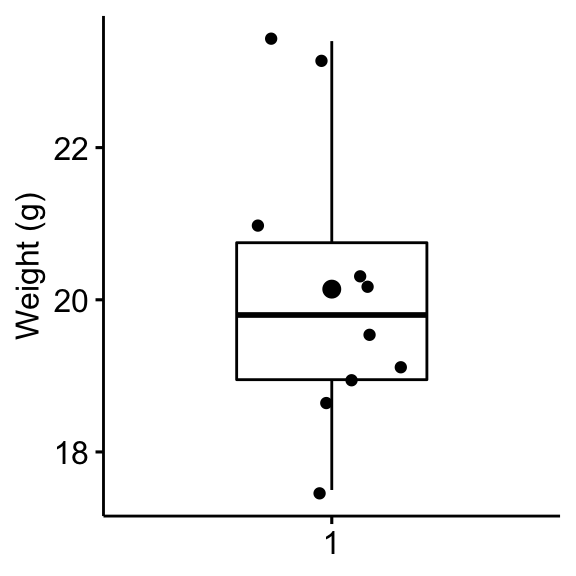
Assumptions and preliminary tests
The Wilcoxon signed-rank test assumes that the data are distributed symmetrically around the median. This can be checked by visual inspection using histogram and density distribution.
Create a histogram: As we have only 10 individuals in our data, we specify the option bins = 4 instead of 30 (default).
gghistogram(mice, x = "weight", y = "..density..",
            fill = "steelblue",bins = 4, add_density = TRUE)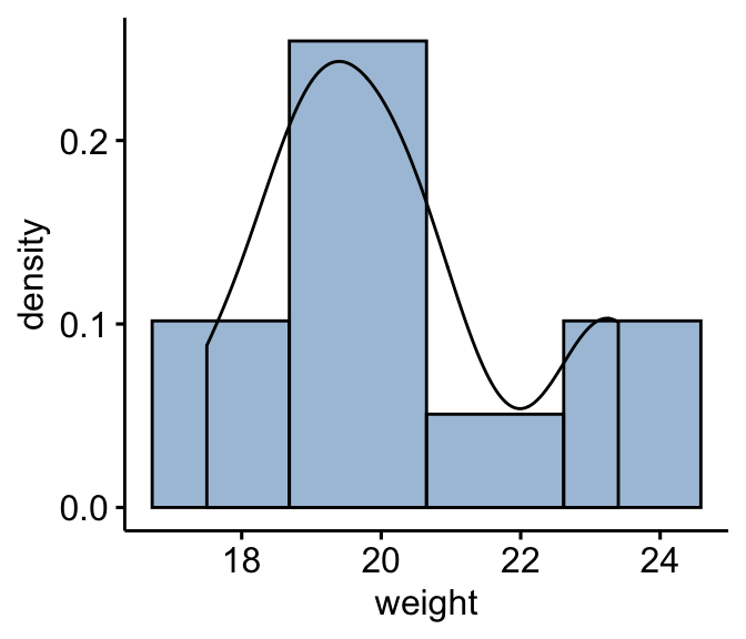
From the plot above, it can be seen that the weight data are approximately symmetrical (you should not expect them to be perfect, particularly when you have smaller numbers of samples in your study). Therefore, we can use the Wilcoxon signed-rank test to analyse our data.
Note that, in the situation where your data is not symmetrically distributed, you could consider performing a sign test, instead of running the Wilcoxon signed-rank test.
The sign test does not make the assumption of a symmetrically-shaped distribution. However, it will most likely be less powerful compared to the Wilcoxon test.
Computation
We want to know, whether the median weight of the mice differs from 25g (two-tailed test)?
stat.test <- mice %>% wilcox_test(weight ~ 1, mu = 25)
stat.test
## # A tibble: 1 x 6
## .y. group1 group2 n statistic p
## * <chr> <chr> <chr> <int> <dbl> <dbl>
## 1 weight 1 null model 10 0 0.00195Note that, to compute one-sided wilcoxon test, you can specify the option alternative, which possible values can be “greater”, “less” or “two.sided”.
Effect size
We’ll use the R function wilcox_effsize() [rstatix]. It requires the coin package for computing the Z statistic.
mice %>% wilcox_effsize(weight ~ 1, mu = 25)## # A tibble: 1 x 6
## .y. group1 group2 effsize n magnitude
## * <chr> <chr> <chr> <dbl> <int> <ord>
## 1 weight 1 null model 0.886 10 largeA large effect size is detected, r = 0.89.
Report
We could report the result as follow:
A Wilcoxon signed-rank test was computed to assess whether the recruited mice median weight was different to the population normal median weight (25g).
The mice weight value were approximately symmetrically distributed, as assessed by a histogram with superimposed density curve.
The measured mice median weight (19.8) was statistically significantly lower than the population median weight 25g (p = 0.002, effect size r = 0.89).
Create a box plot with p-value:
bxp +
  labs(subtitle = get_test_label(stat.test, detailed = TRUE))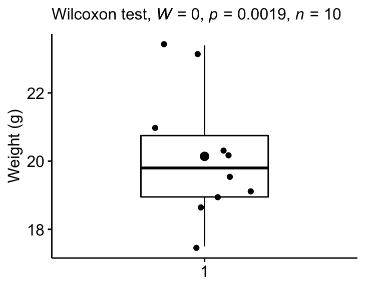
Create a density plot with p-value:
- Red line corresponds to the observed median
- Blue line corresponds to the theoretical median
ggdensity(mice, x = "weight", rug = TRUE, fill = "lightgray") +
  scale_x_continuous(limits = c(15, 27)) +
  stat_central_tendency(type = "median", color = "red", linetype = "dashed") +
  geom_vline(xintercept = 25, color = "blue", linetype = "dashed") +
  labs(subtitle = get_test_label(stat.test, detailed = TRUE))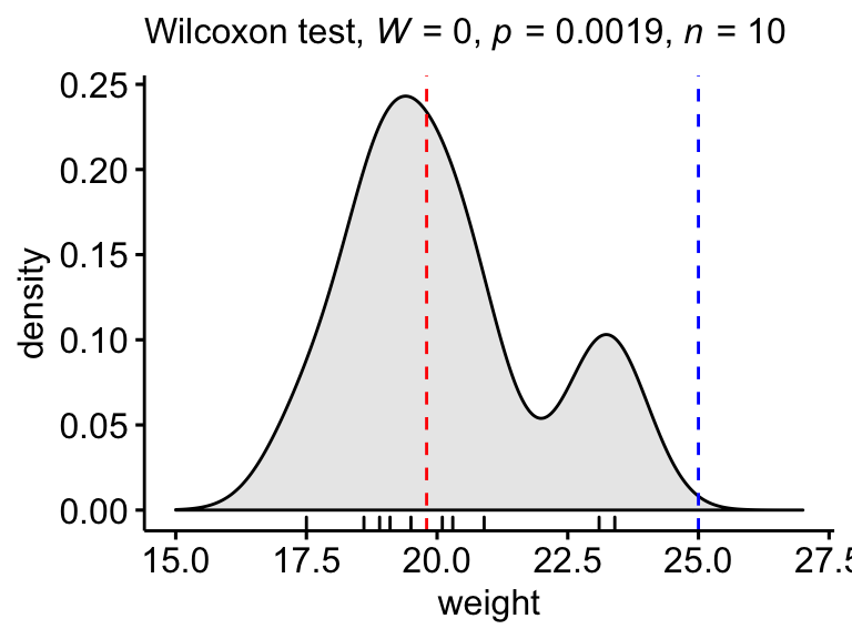
Wilcoxon rank sum test
The Wilcoxon rank sum test is a non-parametric alternative to the independent two samples t-test for comparing two independent groups of samples, in the situation where the data are not normally distributed.
Synonymous: Mann-Whitney test, Mann-Whitney U test, Wilcoxon-Mann-Whitney test and two-sample Wilcoxon test.
Demo data
Demo dataset: genderweight [in datarium package] containing the weight of 40 individuals (20 women and 20 men).
Load the data and show some random rows by groups:
# Load the data
data("genderweight", package = "datarium")
# Show a sample of the data by group
set.seed(123)
genderweight %>% sample_n_by(group, size = 2)
## # A tibble: 4 x 3
## id group weight
## <fct> <fct> <dbl>
## 1 6 F 65.0
## 2 15 F 65.9
## 3 29 M 88.9
## 4 37 M 77.0Summary statistics
Compute some summary statistics by groups: median and interquartile range.
genderweight %>%
  group_by(group) %>%
  get_summary_stats(weight, type = "median_iqr")
## # A tibble: 2 x 5
## group variable n median iqr
## <fct> <chr> <dbl> <dbl> <dbl>
## 1 F weight 20 62.9 2.33
## 2 M weight 20 86.3 4.59Visualization
Visualize the data using box plots. Plot weight by groups.
bxp <- ggboxplot(
  genderweight, x = "group", y = "weight",
  ylab = "Weight", xlab = "Groups", add = "jitter"
  )
bxp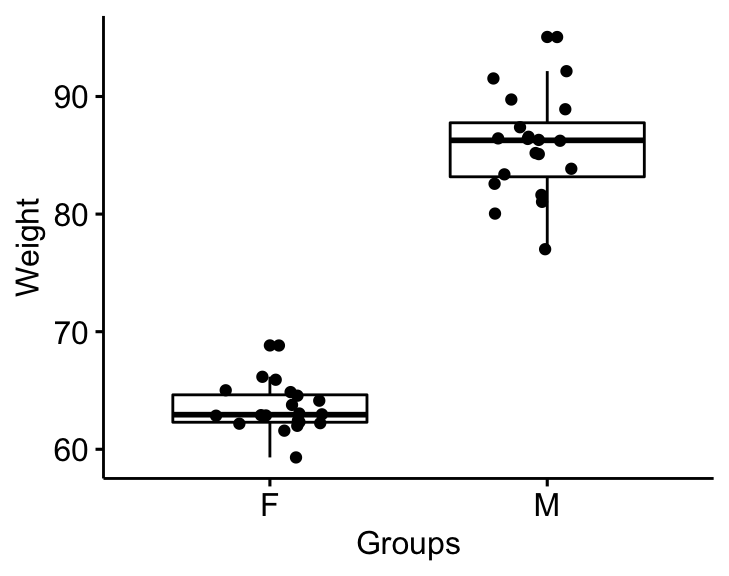
Computation
Question : Is there any significant difference between women and men median weights?
stat.test <- genderweight %>%
  wilcox_test(weight ~ group) %>%
  add_significance()
stat.test
## # A tibble: 1 x 8
## .y. group1 group2 n1 n2 statistic p p.signif
## <chr> <chr> <chr> <int> <int> <dbl> <dbl> <chr>
## 1 weight F M 20 20 0 1.45e-11 ****Effect size
genderweight %>% wilcox_effsize(weight ~ group)## # A tibble: 1 x 7
## .y. group1 group2 effsize n1 n2 magnitude
## * <chr> <chr> <chr> <dbl> <int> <int> <ord>
## 1 weight F M 0.855 20 20 largeA large effect size is detected, r = 0.86.
Report
We could report the result as follow:
The median weight in female group was 62.9 (IQR = 2.33), whereas the median in male group was 86.3 (IQR = 4.59). The Wilcoxon test showed that the difference was significant (p < 0.0001, effect size r = 0.86).
stat.test <- stat.test %>% add_xy_position(x = "group")
bxp +
  stat_pvalue_manual(stat.test, tip.length = 0) +
  labs(subtitle = get_test_label(stat.test, detailed = TRUE))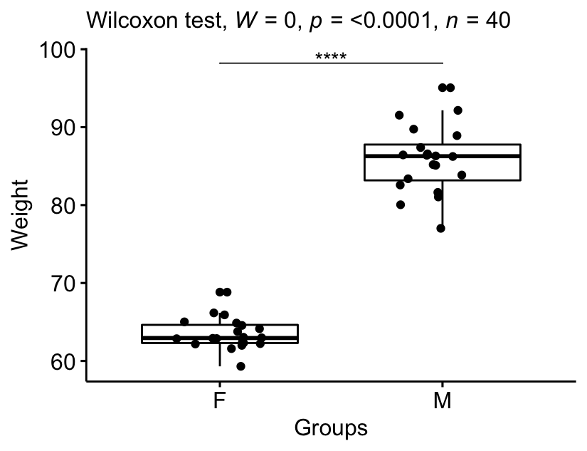
Wilcoxon signed rank test on paired samples
The Wilcoxon signed rank test on paired sample is a non-parametric alternative to the paired samples t-test for comparing paired data. It’s used when the data are not normally distributed.
Demo dataset
Here, we’ll use a demo dataset mice2 [datarium package], which contains the weight of 10 mice before and after the treatment.
# Wide format
data("mice2", package = "datarium")
head(mice2, 3)
## id before after
## 1 1 187 430
## 2 2 194 404
## 3 3 232 406# Transform into long data:
# gather the before and after values in the same column
mice2.long <- mice2 %>%
gather(key = "group", value = "weight", before, after)
head(mice2.long, 3)## id group weight
## 1 1 before 187
## 2 2 before 194
## 3 3 before 232Summary statistics
Compute some summary statistics by groups: median and interquartile range (IQR).
mice2.long %>%
  group_by(group) %>%
  get_summary_stats(weight, type = "median_iqr")
## # A tibble: 2 x 5
## group variable n median iqr
## <chr> <chr> <dbl> <dbl> <dbl>
## 1 after weight 10 405 28.3
## 2 before weight 10 197. 19.2Visualization
bxp <- ggpaired(mice2.long, x = "group", y = "weight",
         order = c("before", "after"),
         ylab = "Weight", xlab = "Groups")
bxp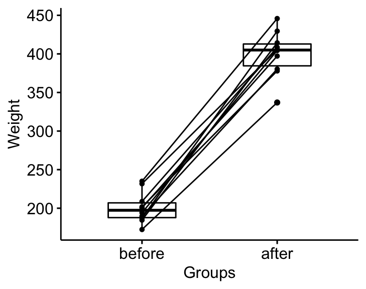
Assumptions and preliminary tests
The test assumes that differences between paired samples should be distributed symmetrically around the median.
Compute the differences between pairs and create histograms:
mice2 <- mice2 %>% mutate(differences = after - before)
gghistogram(mice2, x = "differences", y = "..density..",
            fill = "steelblue",bins = 5, add_density = TRUE)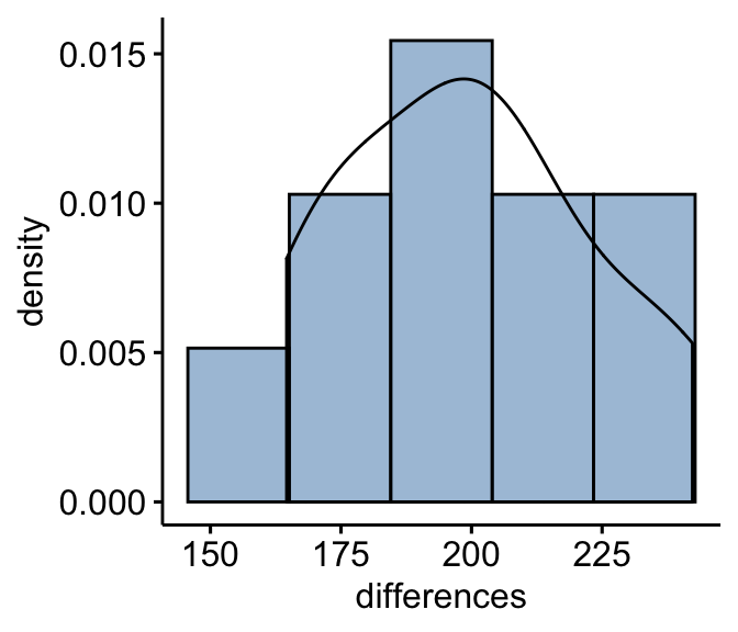
From the plot above, it can be seen that the differences data are approximately symmetrical (you should not expect them to be perfect, particularly when you have smaller numbers of samples in your study). Therefore, we can use the Wilcoxon signed-rank test to analyse our data.
Note that, in the situation where your data is not symmetrically distributed, you could consider performing a sign test, instead of running the Wilcoxon signed-rank test.
The sign test does not make the assumption of a symmetrically-shaped distribution. However, it will most likely be less powerful compared to the Wilcoxon test.
Computation
Question : Is there any significant changes in the weights of mice after treatment?
stat.test <- mice2.long  %>%
  wilcox_test(weight ~ group, paired = TRUE) %>%
  add_significance()
stat.test
## # A tibble: 1 x 8
## .y. group1 group2 n1 n2 statistic p p.signif
## <chr> <chr> <chr> <int> <int> <dbl> <dbl> <chr>
## 1 weight after before 10 10 55 0.00195 **Effect size
mice2.long  %>%
  wilcox_effsize(weight ~ group, paired = TRUE)
## # A tibble: 1 x 7
## .y. group1 group2 effsize n1 n2 magnitude
## * <chr> <chr> <chr> <dbl> <int> <int> <ord>
## 1 weight after before 0.886 10 10 largeA large effect size is detected, r = 0.89.
Report
From the output above, it can be concluded that the median weight of the mice before treatment is significantly different from the median weight after treatment with a p-value = 0.002, effect size r = 0.89.
stat.test <- stat.test %>% add_xy_position(x = "group")
bxp +
  stat_pvalue_manual(stat.test, tip.length = 0) +
  labs(subtitle = get_test_label(stat.test, detailed= TRUE))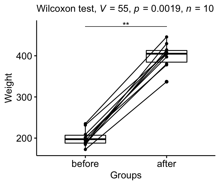
Summary
This chapter describes how to compare two means in R using the Wilcoxon test, which is a non-parametric alternative of the t-test.
Quick start R codes, to compute the different Wilcoxon tests, are:
# One-sample Wilcoxon signed rank test
mice %>% wilcox_test(weight ~ 1, mu = 25)
# Wilcoxon rank sum test: independent samples
genderweight %>% wilcox_test(weight ~ group)
# Wilcoxon signed rank test on paired samples
mice2.long %>% wilcox_test(weight ~ group, paired = TRUE)
Note that, to compute one-sided Wilcoxon tests, you can specify the option alternative, which possible values can be “greater”, “less” or “two.sided”.
Recommended for you
This section contains best data science and self-development resources to help you on your path.
Books - Data Science
Our Books
- Practical Guide to Cluster Analysis in R by A. Kassambara (Datanovia)
- Practical Guide To Principal Component Methods in R by A. Kassambara (Datanovia)
- Machine Learning Essentials: Practical Guide in R by A. Kassambara (Datanovia)
- R Graphics Essentials for Great Data Visualization by A. Kassambara (Datanovia)
- GGPlot2 Essentials for Great Data Visualization in R by A. Kassambara (Datanovia)
- Network Analysis and Visualization in R by A. Kassambara (Datanovia)
- Practical Statistics in R for Comparing Groups: Numerical Variables by A. Kassambara (Datanovia)
- Inter-Rater Reliability Essentials: Practical Guide in R by A. Kassambara (Datanovia)
Others
- R for Data Science: Import, Tidy, Transform, Visualize, and Model Data by Hadley Wickham & Garrett Grolemund
- Hands-On Machine Learning with Scikit-Learn, Keras, and TensorFlow: Concepts, Tools, and Techniques to Build Intelligent Systems by Aurelien Géron
- Practical Statistics for Data Scientists: 50 Essential Concepts by Peter Bruce & Andrew Bruce
- Hands-On Programming with R: Write Your Own Functions And Simulations by Garrett Grolemund & Hadley Wickham
- An Introduction to Statistical Learning: with Applications in R by Gareth James et al.
- Deep Learning with R by François Chollet & J.J. Allaire
- Deep Learning with Python by François Chollet
Version:
 Français

This is amazingly helpful tutorial! I really appreciate it.
Would you mind if I ask one simple question?
It says …
> The Wilcoxon signed-rank test assumes that the data are distributed symmetrically around the median.
I appreciate the way that you introduced a histogram visualization method to test this assumption; however, would there be any way for non-visual learners (i.e., blind people) to test this assumption using R code instead of the visualization technique? I am asking this because I am blind so it would be more than helpful for me to analyze it using R code.
Any advice would be so much appreciated.
Thank you for your positive feedback, highly appreciated.
The function `symmetry.test()` [lawstat packaga] can be used to check whether the data is symmetrically distributed around the median. This function replaces the mean and standard deviation in the classic measure of asymmetry by corresponding robust estimators; the median and mean deviation from the median.
Statistical hypothesis:
– Null hypothesis: the data is symmetric
– Alternative hypothesis: the data is not symmetric
Example of usage:
In the example above, the p-value is not significant (p = 0.4), so we accept the null hypothesis: Our data is symmetrically distributed around the median.
Hi,
Wonderful tutorial, I’ve been following these also from STHDA.
I have troubles using the function: stat_pvalue_manual
Also with the toy data, I get the following error:
Warning: Ignoring unknown aesthetics: xmin, xmax, annotations, y_position
Error in f(…) :
Can only handle data with groups that are plotted on the x-axis
Boxplot is fine all the way to that function, any tips?
Thanks!
Hi,
Please make sure you have the latest version of ggpubr and rstatix
Hi!
Thank you for this tutorial and tutorial about Friedman test; they have been very helpful. Just making a couple of notes:
1. In addition to significance and magnitude, I find it important to know the direction of the difference. In the example at hand, one can see it very clearly even from the boxplots, but generally this is not working. After all, we are dealing with test based on ranks, not the original continuous data. This is why I have used the original wilcoxon.test function to calculate the pseudomedian.
2. Citation from this tutorial: “The Wilcoxon signed-rank test assumes that the data are distributed symmetrically around the median. In other words, there should be roughly the same number of values above and below the median.”
These two phrases are not equivalent. The latter one is always true because of the definition of the median. The first one is what this test truely assumes; if we choose an arbitrary d, the histogram should be about at the same hight in Md – d and Md + d (Md is the median).
Thank you for such a great comments. Following your comments, the improvements below have been made:
Updating the rstatix::wilcox_test() to report an estimator for the pseudomedian (one-sample case) or for the difference of the location parameters x-y. The column estimate and the confidence intervals are now displayed in the test result when the option detailed = TRUE is specified in the
wilcox_test()andpairwise_wilcox_test()functions. You can install the dev version usingdevtools::install_github("kassambara/rstatix")Blog post updated, removing the following sentence “In other words, there should be roughly the same number of values above and below the median”.
Hi Kassambara, please can you also include in the tutorial, how to apply Wilcox test in whole data frame and p.adjusted value. It would be great to see category name/group, p value, q value in columns. I applied pajusted method but i couldn’t see the q value.
Thanks
Hi, I’m not sure to understand what do you means by “apply wilcox test in whol data frame”? Do you want to apply the test for each variable in the data frame?
Yes, E.g. comparing 100’s of genes/proteins/bacteria between two groups is tough to do one by one. It would be good if p value can be calculated for all at one time. Maybe using apply or something. Also important to add FDR correction.
See this link, somebody asked in stackoverflow.
https://stackoverflow.com/questions/21271449/how-to-apply-the-wilcox-test-to-a-whole-dataframe-in-r
Thanks
Hi!
Thank you for this tutorial. I found it very useful. I have a question about the effect size. All of the examples above have a large effect size, but I still don’t understand what this means. Can you please get in details what is the impact of the effect size?
I really appreciate this tutorial. However, whenever I try to reproduce the Wilcoxon test, the following appears:
Error in UseMethod(“wilcox_test”) : no applicable method for ‘wilcox_test’ applied to an object of class “data.frame”
This occurred with my own data, but I also tried it with the “Toothgrowth” example above and got the same error message.
Could you please clarify the issue?
I am coming across the same error. Can anyone help with this?
I’m getting this error now even though it was working for me this morning. what gives?
I solved it today. I think there might be other packages in conflict so you can work around it by specifying the rstatix package:
rstatix::wilcox_test()
Thank you!!!! Now it wokrs
Thank you !!
I wrote following and it works perfectly!
Wilc_Mean % rstatix::wilcox_test(Mean_HOR ~ Mean_MYG, paired = TRUE)
Hello. I tried the Wilcoxon signed rank test on paired samples as described here, and by using GraphPad Prism. I do not get the same result. How does the wilcox_test deal with cases where there has been no change from before to after? And how does it handle zero’s? For exampled that you looked at the relative abundance of some bacteria in 30 people before and after some treatment. But then you have a couple of people that did not change at all, or you have some people that had 0 abundance before and still 0 abundance after. Thanks
No assumptions check for the standard Wilcoxon one?
It’s worth mentioning, that the stochastic equivalence is a general term and isn’t limited only to the shift in location. You may have perfectly equal medians and it will reject H0 if the dispersions vary. That’s why it’s not a test of medians, but rather pseudo medians, which approach medians, as the data get symmetric and have equal dispersion. You mention the pseudomedians, that’s very good! I write it just because many, many people treat the MW(W) test as a test of medians (or median difference), which *approximates* it only in a certain, special and quite rare case. As the famous article says (can be googled in seconds): “Mann-Whitney fails as a test of medians”. Same about the Kruskal-Wallis or Friedman.
Hi,
thank you for this tutorial
I’m a bit confused since the title and subtitles talk about mean comparison but everywhere else inside the tutorial it seems that these tests are used for median comparison. Could this be fixed or explained?
Thanks!
I know that the pairing is done between the first x and y pair, however, we often have long data formats that are not necessarily ordered in a way that this pairing makes sense. Could I include ID in the analysis to ensure the pairings are made correctly without too much manual work on the data frame?
Many thanks for considering my request.
yes, this!
It would be a relief to know that it was finding the correct pairs through the analysis.