R is a free and powerful statistical software for analyzing and visualizing data. If you want to learn easily the essential of R programming, visit our series of tutorials available on STHDA: http://www.sthda.com/english/wiki/r-basics-quick-and-easy.
In this chapter, you will learn:
- a very brief introduction to R, for installing R/RStudio as well as importing your data into R and installing required libraries.
- introduction to categorical data structure
- basics of creating contingency tables
Contents:
Related Book
Inter-Rater Reliability Essentials: Practical Guide in RInstall R and RStudio
Standard installation
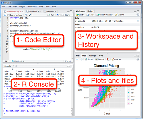
R and RStudio can be installed on Windows, MAC OSX and Linux platforms. RStudio is an integrated development environment for R that makes using R easier. It includes a console, code editor and tools for plotting.
- R can be downloaded and installed from the Comprehensive R Archive Network (CRAN) webpage (http://cran.r-project.org/)
- After installing R software, install also the RStudio software available at: http://www.rstudio.com/products/RStudio/.
- Launch RStudio and start use R inside R studio.
R Online
R can be also accessed online without any installation. You can find an example at https://rdrr.io/snippets/. This site include thousands add-on packages.
Install and load required R packages
An R package is a collection of functionalities that extends the capabilities of base R. For example, to use the R code provided in this book, you should install the following R packages:
tidyversepackages, which are a collection of R packages that share the same programming philosophy. These packages include:readr: for importing data into Rdplyr: for data manipulationggplot2: for data visualization.
datarium: contains demo data for statistical analyses.irr,vcdand thepsychpackages: for inter-rater reliability measures. which makes it easy, for beginner, to create publication ready plots
- Install the tidyverse package. Installing tidyverse will install automatically readr, dplyr, ggplot2 and more. Type the following code in the R console:
install.packages("tidyverse")- Install datarium, irr, vcd and psych
install.packages("datarium")
install.packages("irr")
install.packages("vcd")
install.packages("psych")- Load required packages. After installation, you must first load the package for using the functions in the package. The function
library()is used for this task. An alternative function isrequire(). For example, to load thevcdpackage, type this:
library("vcd")Now, we can use R functions, such as Kappa() [in the vcd package] for computing Cohen’s Kappa and weighted kappa.
If you want a help about a given function, say Kappa(), type this in R console: ?Kappa.
Data format
Your data should be in rectangular format, where columns are variables and rows are observations (individuals or samples).
- Column names should be compatible with R naming conventions. Avoid column with blank space and special characters. Good column names:
long_jumporlong.jump. Bad column name:long jump. - Avoid beginning column names with a number. Use letter instead. Good column names:
sport_100morx100m. Bad column name:100m. - Replace missing values by
NA(for not available)
For example, your data should look like this:
Read more at: Best Practices in Preparing Data Files for Importing into R
Import your data in R
First, save your data into txt or csv file formats and import it as follow (you will be asked to choose the file):
library("readr")

# Reads tab delimited files (.txt tab)
my_data <- read_tsv(file.choose())

# Reads comma (,) delimited files (.csv)
my_data <- read_csv(file.choose())

# Reads semicolon(;) separated files(.csv)
my_data <- read_csv2(file.choose())
Read more about how to import data into R at this link: http://www.sthda.com/english/wiki/importing-data-into-r
Demo data sets
R comes with several demo data sets for playing with R functions. The most used R demo data sets include: USArrests, iris and mtcars. To load a demo data set, use the function data() as follow. The function head() is used to inspect the data.
data("iris")   # Loading
head(iris, n = 3)  # Print the first n = 3 rows
## Sepal.Length Sepal.Width Petal.Length Petal.Width Species
## 1 5.1 3.5 1.4 0.2 setosa
## 2 4.9 3.0 1.4 0.2 setosa
## 3 4.7 3.2 1.3 0.2 setosaTo learn more about iris data sets, type this:
?irisAfter typing the above R code, you will see the description of iris data set: this iris data set gives the measurements in centimeters of the variables sepal length and width and petal length and width, respectively, for 50 flowers from each of 3 species of iris. The species are Iris setosa, versicolor, and virginica.
Data manipulation
After importing your data in R, you can easily manipulate it using the dplyr package, which can be installed using the R code: install.packages("dplyr").
After loading dplyr, you can use the following R functions:
filter(): Pick rows (observations/samples) based on their values.distinct(): Remove duplicate rows.arrange(): Reorder the rows.select(): Select columns (variables) by their names.rename(): Rename columns.mutate(): Add/create new variables.summarise(): Compute statistical summaries (e.g., computing the mean or the sum)group_by(): Operate on subsets of the data set.
Note that, dplyr package allows to use the forward-pipe chaining operator (%>%) for combining multiple operations. For example, x %>% f is equivalent to f(x). Using the pipe (%>%), the output of each operation is passed to the next operation. This makes R programming easy.
Read more about Data Manipulation at this link: https://www.datanovia.com/en/courses/data-manipulation-in-r/
Working with Categorical data
Definition
Categorical variables are variables whose values comprise a set of groups. Examples of categorical variables include: gender (male, female), passenger’s classes (1st, 2nd, 3rd class), smokers (yes, no), eye color (brown, blue, Hazel, Green) etc.
There are different types of categorical variables depending on the number of categories they contain:
- Binary variables or dichotomous variables contain only two groups
- Polytomous variables contain three or more groups
Categorical variables containing ordered categories, such as passenger’s classes (1st < 2nd < 3rd), are called ordinal variables. Categorical variable containing unordered categories, such as eye color (brown, blue, Hazel, Green), are called nominal variable.
Data structure
Categorical data can be available into different forms, including:
- Case form, in which each row corresponds to a case (or individual)
- Frequency form, in which the data are tabulated. The table cells contain the frequencies of categories (cross-classified or not).
Example of case form: HairEyeColor data
##    Hair   Eye
## 1 Black Brown
## 2 Black Brown
## 3 Black Brown
## 4 Black Brown
Example of frequency form (1/2) : Cross-tabulation
##        Eye
## Hair    Brown Blue Hazel Green
##   Black    32   11    10     3
##   Brown    53   50    25    15
##   Red      10   10     7     7
##   Blond     3   30     5     8
Example of frequency form (2/2) : Data frame
##    Hair   Eye Freq
## 1 Black Brown   32
## 2 Brown Brown   53
## 3   Red Brown   10
## 4 Blond Brown    3
Create contingency table
This section describes how to create contingency table in R. You will learn how to:
- Create one-, two- and three-way tables containing the frequency counts
- Compute proportions and, add rows and columns totals
- Transform a multi-way contingency table into a beautiful two-way flat format
- Subset a contingency table
Input Data
data("titanic.raw", package = "datarium")
head(titanic.raw)
## Class Sex Age Survived
## 1 3rd Male Child No
## 2 3rd Male Child No
## 3 3rd Male Child No
## 4 3rd Male Child No
## 5 3rd Male Child No
## 6 3rd Male Child NoKey R functions
table()andxtabs(): Create contingency tables containing frequencies.xtabsallows to use formulas.prop.table(): Compute proportions over rows, columns or overall totalsmargin.table(): Compute rows, columns or overall totals (i.e, sums)
Create contingency tables
Using xtabs(): formula interface
# One way table
xtabs(~Class, data = titanic.raw)
## Class
## 1st 2nd 3rd Crew
## 325 285 706 885# Two way table
xtabs(~Class + Survived, data = titanic.raw)## Survived
## Class No Yes
## 1st 122 203
## 2nd 167 118
## 3rd 528 178
## Crew 673 212# Three way table
xtabs(~Class + Survived + Sex, data = titanic.raw)## , , Sex = Male
##
## Survived
## Class No Yes
## 1st 118 62
## 2nd 154 25
## 3rd 422 88
## Crew 670 192
##
## , , Sex = Female
##
## Survived
## Class No Yes
## 1st 4 141
## 2nd 13 93
## 3rd 106 90
## Crew 3 20Using table()
# One way table -----------
# use this:
table(titanic.raw$Class)
# Or this
table(titanic.raw[, "Class"])
# or this:
with(titanic.raw, table(Class))

# Two way table -----------
with(titanic.raw, table(Class, Survived))

# Three way table -----------
with(titanic.raw, table(Class, Survived, Sex))
Compute margins: row and column totals
# Two way table
xtab <- xtabs(~Class + Survived, data = titanic.raw)
# Compute row totals
margin.table(xtab, 1)
## Class
## 1st 2nd 3rd Crew
## 325 285 706 885# Compute column totals
margin.table(xtab, 2)## Survived
## No Yes
## 1490 711You can also use the functions rowSums() and colSums().
Add rows and columns sums to the table
addmargins(xtab)## Survived
## Class No Yes Sum
## 1st 122 203 325
## 2nd 167 118 285
## 3rd 528 178 706
## Crew 673 212 885
## Sum 1490 711 2201Compue proportions
# Frequencies relative to row total
prop.table(xtab, 1)
## Survived
## Class No Yes
## 1st 0.375 0.625
## 2nd 0.586 0.414
## 3rd 0.748 0.252
## Crew 0.760 0.240# Frequencies relative to column total
prop.table(xtab, 2)## Survived
## Class No Yes
## 1st 0.0819 0.2855
## 2nd 0.1121 0.1660
## 3rd 0.3544 0.2504
## Crew 0.4517 0.2982# Frequencies relative to the table grand total
xtab/sum(xtab)## Survived
## Class No Yes
## 1st 0.0554 0.0922
## 2nd 0.0759 0.0536
## 3rd 0.2399 0.0809
## Crew 0.3058 0.0963Close your R/RStudio session
Each time you close R/RStudio, you will be asked whether you want to save the data from your R session. If you decide to save, the data will be available in future R sessions.
Summary
This chapter provides a quick introduction to R and a brief description of how to work with categorical data in R.
Recommended for you
This section contains best data science and self-development resources to help you on your path.
Books - Data Science
Our Books
- Practical Guide to Cluster Analysis in R by A. Kassambara (Datanovia)
- Practical Guide To Principal Component Methods in R by A. Kassambara (Datanovia)
- Machine Learning Essentials: Practical Guide in R by A. Kassambara (Datanovia)
- R Graphics Essentials for Great Data Visualization by A. Kassambara (Datanovia)
- GGPlot2 Essentials for Great Data Visualization in R by A. Kassambara (Datanovia)
- Network Analysis and Visualization in R by A. Kassambara (Datanovia)
- Practical Statistics in R for Comparing Groups: Numerical Variables by A. Kassambara (Datanovia)
- Inter-Rater Reliability Essentials: Practical Guide in R by A. Kassambara (Datanovia)
Others
- R for Data Science: Import, Tidy, Transform, Visualize, and Model Data by Hadley Wickham & Garrett Grolemund
- Hands-On Machine Learning with Scikit-Learn, Keras, and TensorFlow: Concepts, Tools, and Techniques to Build Intelligent Systems by Aurelien Géron
- Practical Statistics for Data Scientists: 50 Essential Concepts by Peter Bruce & Andrew Bruce
- Hands-On Programming with R: Write Your Own Functions And Simulations by Garrett Grolemund & Hadley Wickham
- An Introduction to Statistical Learning: with Applications in R by Gareth James et al.
- Deep Learning with R by François Chollet & J.J. Allaire
- Deep Learning with Python by François Chollet
Version:
 Français

No Comments