Easy Correlation Matrix Analysis in R Using Corrr Package

Load required R packages

• tidyverse: easy data manipulation and visualization
• corrr: correlation matrix analysis

library(tidyverse)  
library(corrr)

Data preparation

# Select columns of interest
mydata <- mtcars %>% 
  select(mpg, disp, hp, drat, wt, qsec)
# Add some missing values
mydata$hp[3] <- NA
# Inspect the data
head(mydata, 3)

##                mpg disp  hp drat   wt qsec
## Mazda RX4     21.0  160 110 3.90 2.62 16.5
## Mazda RX4 Wag 21.0  160 110 3.90 2.88 17.0
## Datsun 710    22.8  108  NA 3.85 2.32 18.6

Compute correlation matrix

Key R function: correlate(), which is a wrapper around the cor() R base function but with the following advantages:

• Handles missing values by default with the optionuse = "pairwise.complete.obs"
• Diagonal values is set to NA, so that it can be easily removed
• Returns a data frame, which can be easily manipulated using the tidyverse package.

library(corrr)
res.cor <- correlate(mydata)
res.cor

## # A tibble: 6 x 7
##   rowname     mpg    disp      hp     drat      wt     qsec
##   <chr>     <dbl>   <dbl>   <dbl>    <dbl>   <dbl>    <dbl>
## 1 mpg      NA      -0.848  -0.775   0.681   -0.868   0.419 
## 2 disp     -0.848  NA       0.786  -0.710    0.888  -0.434 
## 3 hp       -0.775   0.786  NA      -0.443    0.651  -0.706 
## 4 drat      0.681  -0.710  -0.443  NA       -0.712   0.0912
## 5 wt       -0.868   0.888   0.651  -0.712   NA      -0.175 
## 6 qsec      0.419  -0.434  -0.706   0.0912  -0.175  NA

Additional arguments for the function correlate(), include:

• method: a character string indicating which correlation coefficient (or covariance) is to be computed. One of “pearson” (default), “kendall”, or “spearman”: can be abbreviated.
• diagonal: Value (typically numeric or NA) to set the diagonal to.

For example, type this:

correlate(mydata, method = "spearman", diagonal = 1)

Key corrr functions for exploring correlation matrix

The corrr R package comes also with some key functions facilitating the exploration of the correlation matrix. Here’s a diagram showing the primary corrr functions:

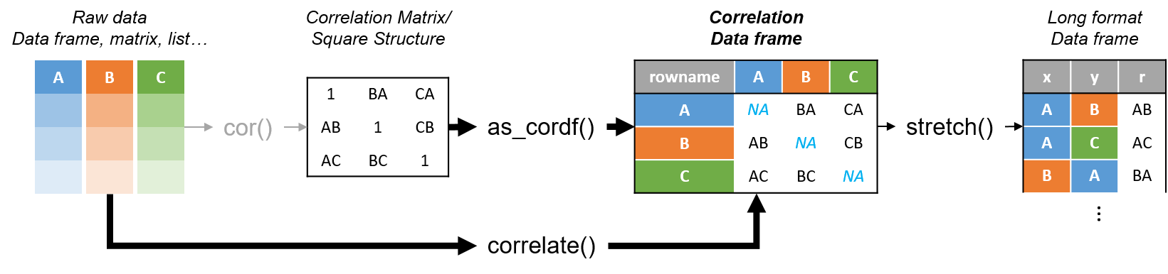
The corrr API is designed with data pipelines in mind (e.g., to use %>% from the magrittr package). After correlate(), the primary corrr functions take a cor_df as their first argument, and return a cor_df or tbl (or output like a plot). These functions serve one of three purposes:

Internal changes (cor_df out):

• shave() the upper or lower triangle (set to NA).
• rearrange() the columns and rows based on correlation strengths.

Reshape structure (tbl or cor_df out):

• focus() on select columns and rows.
• stretch() into a long format.

Output/visualisations (console/plot out):

• fashion() the correlations for pretty printing.
• rplot() the correlations with shapes in place of the values.
• network_plot() the correlations in a network.

You can also easily manipulate the correlation results using the tidyverse verbs. For example, filter correlations above 0.8:

res.cor %>%  
  gather(-rowname, key = "colname", value = "cor") %>% 
  filter(abs(cor) > 0.8)

## # A tibble: 6 x 3
##   rowname colname    cor
##   <chr>   <chr>    <dbl>
## 1 disp    mpg     -0.848
## 2 wt      mpg     -0.868
## 3 mpg     disp    -0.848
## 4 wt      disp     0.888
## 5 mpg     wt      -0.868
## 6 disp    wt       0.888

Focus on specific columns/rows

The function focus() makes it possible to focus() on columns and rows. This function acts just like dplyr’s select(), but also excludes the selected columns from the rows (or everything else with the mirror argument).

• Select correlation results with columns of interests. The selected columns are excluded from the rows:

res.cor %>% 
  focus(mpg, disp, hp)

## # A tibble: 3 x 4
##   rowname    mpg   disp     hp
##   <chr>    <dbl>  <dbl>  <dbl>
## 1 drat     0.681 -0.710 -0.443
## 2 wt      -0.868  0.888  0.651
## 3 qsec     0.419 -0.434 -0.706

• Mirror the selected columns:

res.cor %>% 
  focus(mpg, disp, hp, mirror = TRUE)

## # A tibble: 3 x 4
##   rowname     mpg    disp      hp
##   <chr>     <dbl>   <dbl>   <dbl>
## 1 mpg      NA      -0.848  -0.775
## 2 disp     -0.848  NA       0.786
## 3 hp       -0.775   0.786  NA

• Remove unwanted columns:

res.cor %>% 
  focus(-mpg, -disp, -hp)

## # A tibble: 3 x 4
##   rowname   drat     wt   qsec
##   <chr>    <dbl>  <dbl>  <dbl>
## 1 mpg      0.681 -0.868  0.419
## 2 disp    -0.710  0.888 -0.434
## 3 hp      -0.443  0.651 -0.706

• Select columns by regular expression

res.cor %>% 
  focus(matches("^d"))

## # A tibble: 4 x 3
##   rowname   disp    drat
##   <chr>    <dbl>   <dbl>
## 1 mpg     -0.848  0.681 
## 2 hp       0.786 -0.443 
## 3 wt       0.888 -0.712 
## 4 qsec    -0.434  0.0912

• Select correlation above 0.8:

any_over_90 <- function(x) any(x > .8, na.rm = TRUE)
res.cor %>% 
  focus_if(any_over_90, mirror = TRUE)

## # A tibble: 2 x 3
##   rowname   disp     wt
##   <chr>    <dbl>  <dbl>
## 1 disp    NA      0.888
## 2 wt       0.888 NA

• Focus on correlations of one variable with all others:

# Extract the correlation
res.cor %>% 
  focus(mpg)

## # A tibble: 5 x 2
##   rowname    mpg
##   <chr>    <dbl>
## 1 disp    -0.848
## 2 hp      -0.775
## 3 drat     0.681
## 4 wt      -0.868
## 5 qsec     0.419

# Plot the correlation between mpg and all others
res.cor %>%
  focus(mpg) %>%
  mutate(rowname = reorder(rowname, mpg)) %>%
  ggplot(aes(rowname, mpg)) +
    geom_col() + coord_flip() +
  theme_bw()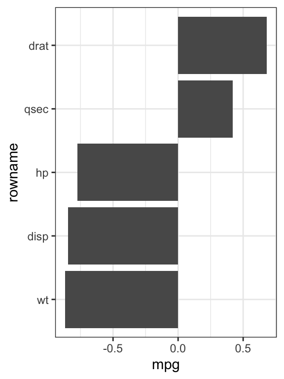

Reorder the correlation matrix

You can also rearrange() the entire data frame based on clustering algorithms:

res.cor %>% rearrange()

## # A tibble: 6 x 7
##   rowname      wt     drat    disp     mpg      hp     qsec
##   <chr>     <dbl>    <dbl>   <dbl>   <dbl>   <dbl>    <dbl>
## 1 wt       NA      -0.712    0.888  -0.868   0.651  -0.175 
## 2 drat     -0.712  NA       -0.710   0.681  -0.443   0.0912
## 3 disp      0.888  -0.710   NA      -0.848   0.786  -0.434 
## 4 mpg      -0.868   0.681   -0.848  NA      -0.775   0.419 
## 5 hp        0.651  -0.443    0.786  -0.775  NA      -0.706 
## 6 qsec     -0.175   0.0912  -0.434   0.419  -0.706  NA

Shave off upper/lower triangle

shave() the upper/lower triangle to missing values

res.cor %>% shave()

## # A tibble: 6 x 7
##   rowname     mpg    disp      hp     drat      wt  qsec
##   <chr>     <dbl>   <dbl>   <dbl>    <dbl>   <dbl> <dbl>
## 1 mpg      NA      NA      NA      NA       NA        NA
## 2 disp     -0.848  NA      NA      NA       NA        NA
## 3 hp       -0.775   0.786  NA      NA       NA        NA
## 4 drat      0.681  -0.710  -0.443  NA       NA        NA
## 5 wt       -0.868   0.888   0.651  -0.712   NA        NA
## 6 qsec      0.419  -0.434  -0.706   0.0912  -0.175    NA

Stretch correlation data frame into long format

res.cor %>% stretch()

## # A tibble: 36 x 3
##   x     y           r
##   <chr> <chr>   <dbl>
## 1 mpg   mpg    NA    
## 2 mpg   disp   -0.848
## 3 mpg   hp     -0.775
## 4 mpg   drat    0.681
## 5 mpg   wt     -0.868
## 6 mpg   qsec    0.419
## # … with 30 more rows

Manipulate the correlations using both tidyverse and corrr packages

Visualize the distribution of the correlation coefficients:

res.cor %>%
  shave() %>% 
  stretch(na.rm = TRUE) %>% 
  ggplot(aes(r)) +
    geom_histogram(bins = 10)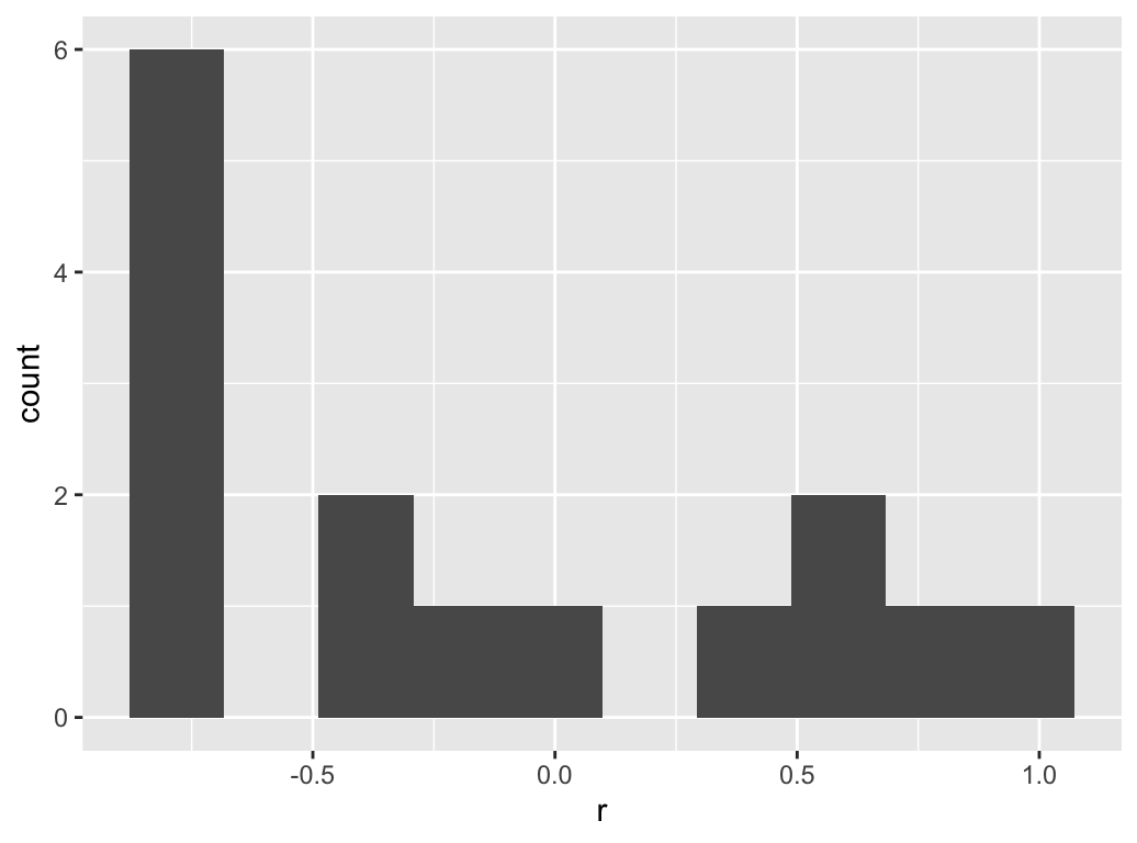

Rearrange and filter the correlation matrix:

res.cor %>%
  focus(mpg:drat, mirror = TRUE) %>% 
  rearrange() %>% 
  shave(upper = FALSE) %>% 
  select(-hp) %>% 
  filter(rowname != "drat")

## # A tibble: 3 x 4
##   rowname     mpg    disp   drat
##   <chr>     <dbl>   <dbl>  <dbl>
## 1 hp       -0.775   0.786 -0.443
## 2 mpg      NA      -0.848  0.681
## 3 disp     NA      NA     -0.710

Viualize and interpret the correlations

• fashionable correlations:

res.cor %>% fashion()

##   rowname  mpg disp   hp drat   wt qsec
## 1     mpg      -.85 -.77  .68 -.87  .42
## 2    disp -.85       .79 -.71  .89 -.43
## 3      hp -.77  .79      -.44  .65 -.71
## 4    drat  .68 -.71 -.44      -.71  .09
## 5      wt -.87  .89  .65 -.71      -.17
## 6    qsec  .42 -.43 -.71  .09 -.17

res.cor %>%
  focus(mpg:drat, mirror = TRUE) %>% 
  rearrange() %>% 
  shave(upper = FALSE) %>% 
  select(-hp) %>% 
  filter(rowname != "drat") %>% 
  fashion()

##   rowname  mpg disp drat
## 1      hp -.77  .79 -.44
## 2     mpg      -.85  .68
## 3    disp           -.71

• Make a correlogram using rplot():

res.cor %>% rplot()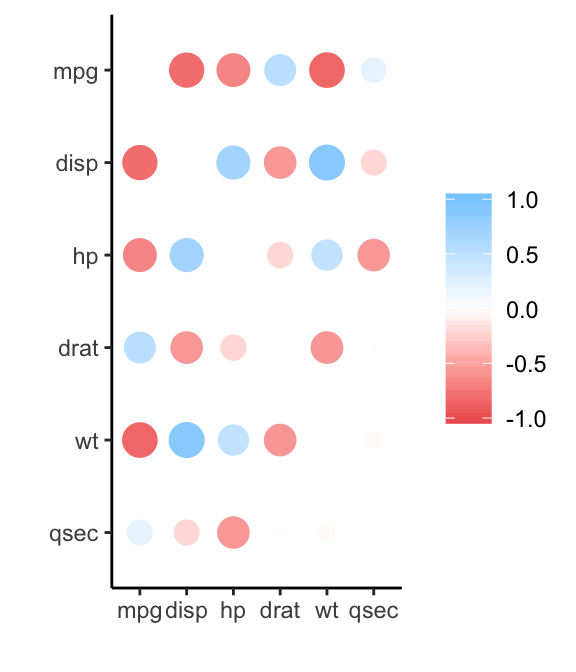

• Rearrange and then plot the lower triangle:

res.cor %>%
  rearrange(method = "MDS", absolute = FALSE) %>%
  shave() %>% 
  rplot(shape = 15, colours = c("red", "green"))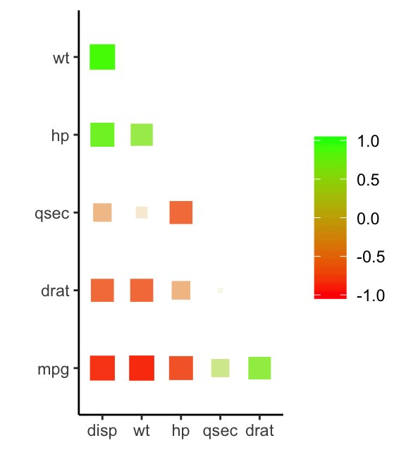

• Make a network plot

res.cor %>% network_plot(min_cor = .6)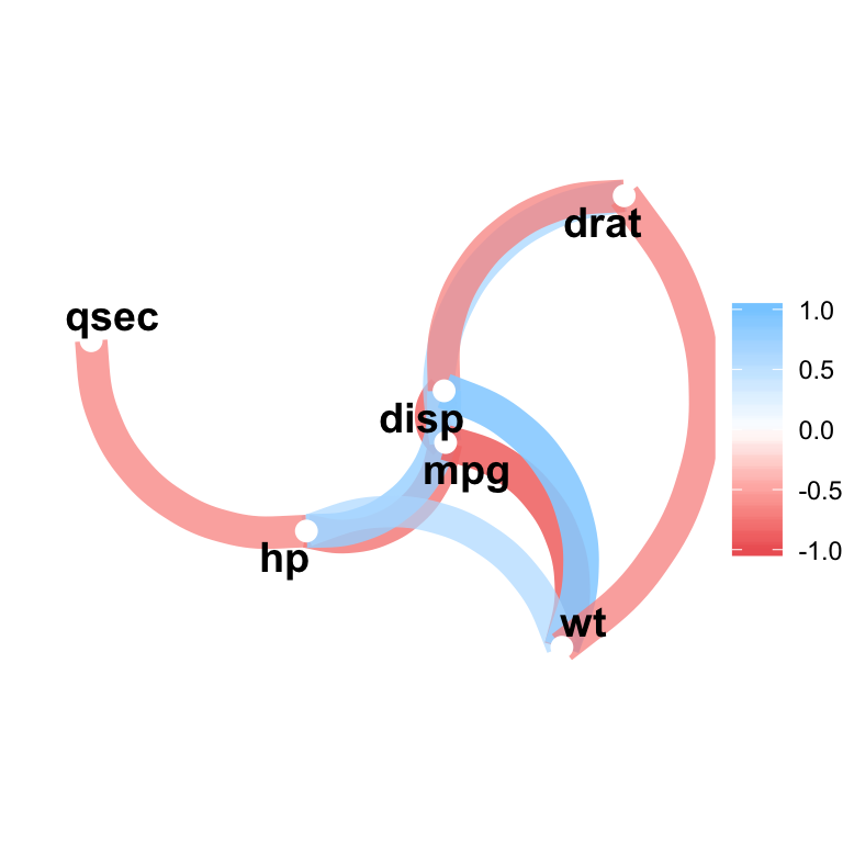

Correlate data in databases

• Using SQLite database:

con <- DBI::dbConnect(RSQLite::SQLite(), path = ":dbname:")
db_mtcars <- copy_to(con, mtcars)
class(db_mtcars)

correlate() detects DB backend, uses tidyeval to calculate correlations in the database, and returns correlation data frame.

db_mtcars %>% correlate(use = "complete.obs")

• Using spark:

sc <- sparklyr::spark_connect(master = "local")
mtcars_tbl <- copy_to(sc, mtcars)
correlate(mtcars_tbl, use = "complete.obs")

Reference

• Exploring correlations in R with corrr