The ANOVA test (or Analysis of Variance) is used to compare the mean of multiple groups. The term ANOVA is a little misleading. Although the name of the technique refers to variances, the main goal of ANOVA is to investigate differences in means.
This chapter describes the different types of ANOVA for comparing independent groups, including:
- One-way ANOVA: an extension of the independent samples t-test for comparing the means in a situation where there are more than two groups. This is the simplest case of ANOVA test where the data are organized into several groups according to only one single grouping variable (also called factor variable). Other synonyms are: 1 way ANOVA, one-factor ANOVA and between-subject ANOVA.
- two-way ANOVA used to evaluate simultaneously the effect of two different grouping variables on a continuous outcome variable. Other synonyms are: two factorial design, factorial anova or two-way between-subjects ANOVA.
- three-way ANOVA used to evaluate simultaneously the effect of three different grouping variables on a continuous outcome variable. Other synonyms are: factorial ANOVA or three-way between-subjects ANOVA.
Note that, the independent grouping variables are also known as between-subjects factors.
The main goal of two-way and three-way ANOVA is, respectively, to evaluate if there is a statistically significant interaction effect between two and three between-subjects factors in explaining a continuous outcome variable.
You will learn how to:
- Compute and interpret the different types of ANOVA in R for comparing independent groups.
- Check ANOVA test assumptions
- Perform post-hoc tests, multiple pairwise comparisons between groups to identify which groups are different
- Visualize the data using box plots, add ANOVA and pairwise comparisons p-values to the plot
Contents:
Related Book
Practical Statistics in R II - Comparing Groups: Numerical VariablesBasics
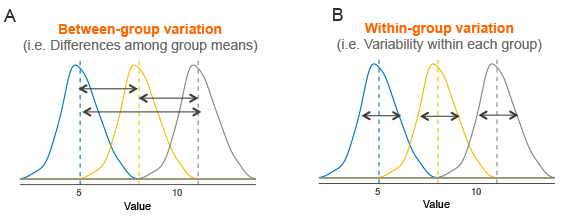
Assume that we have 3 groups to compare, as illustrated in the image below. The dashed line indicates the group mean. The figure shows the variation between the means of the groups (panel A) and the variation within each group (panel B), also known as residual variance.
The idea behind the ANOVA test is very simple: if the average variation between groups is large enough compared to the average variation within groups, then you could conclude that at least one group mean is not equal to the others.
Thus, it’s possible to evaluate whether the differences between the group means are significant by comparing the two variance estimates. This is why the method is called analysis of variance even though the main goal is to compare the group means.
Briefly, the mathematical procedure behind the ANOVA test is as follow:
- Compute the within-group variance, also known as residual variance. This tells us, how different each participant is from their own group mean (see figure, panel B).
- Compute the variance between group means (see figure, panel A).
- Produce the F-statistic as the ratio of
variance.between.groups/variance.within.groups.
Note that, a lower F value (F < 1) indicates that there are no significant difference between the means of the samples being compared.
However, a higher ratio implies that the variation among group means are greatly different from each other compared to the variation of the individual observations in each groups.
Assumptions
The ANOVA test makes the following assumptions about the data:
- Independence of the observations. Each subject should belong to only one group. There is no relationship between the observations in each group. Having repeated measures for the same participants is not allowed.
- No significant outliers in any cell of the design
- Normality. the data for each design cell should be approximately normally distributed.
- Homogeneity of variances. The variance of the outcome variable should be equal in every cell of the design.
Before computing ANOVA test, you need to perform some preliminary tests to check if the assumptions are met.
Note that, if the above assumptions are not met there are a non-parametric alternative (Kruskal-Wallis test) to the one-way ANOVA.
Unfortunately, there are no non-parametric alternatives to the two-way and the three-way ANOVA. Thus, in the situation where the assumptions are not met, you could consider running the two-way/three-way ANOVA on the transformed and non-transformed data to see if there are any meaningful differences.
If both tests lead you to the same conclusions, you might not choose to transform the outcome variable and carry on with the two-way/three-way ANOVA on the original data.
It’s also possible to perform robust ANOVA test using the WRS2 R package.
No matter your choice, you should report what you did in your results.
Prerequisites
Make sure you have the following R packages:
tidyversefor data manipulation and visualizationggpubrfor creating easily publication ready plotsrstatixprovides pipe-friendly R functions for easy statistical analysesdatarium: contains required data sets for this chapter
Load required R packages:
library(tidyverse)
library(ggpubr)
library(rstatix)
Key R functions: anova_test() [rstatix package], wrapper around the function car::Anova().
One-way ANOVA
Data preparation
Here, we’ll use the built-in R data set named PlantGrowth. It contains the weight of plants obtained under a control and two different treatment conditions.
Load and inspect the data by using the function sample_n_by() to display one random row by groups:
data("PlantGrowth")
set.seed(1234)
PlantGrowth %>% sample_n_by(group, size = 1)
## # A tibble: 3 x 2
## weight group
## <dbl> <fct>
## 1 5.58 ctrl
## 2 6.03 trt1
## 3 4.92 trt2Show the levels of the grouping variable:
levels(PlantGrowth$group)## [1] "ctrl" "trt1" "trt2"If the levels are not automatically in the correct order, re-order them as follow:
PlantGrowth <- PlantGrowth %>%
  reorder_levels(group, order = c("ctrl", "trt1", "trt2"))
The one-way ANOVA can be used to determine whether the means plant growths are significantly different between the three conditions.
Summary statistics
Compute some summary statistics (count, mean and sd) of the variable weight organized by groups:
PlantGrowth %>%
  group_by(group) %>%
  get_summary_stats(weight, type = "mean_sd")
## # A tibble: 3 x 5
## group variable n mean sd
## <fct> <chr> <dbl> <dbl> <dbl>
## 1 ctrl weight 10 5.03 0.583
## 2 trt1 weight 10 4.66 0.794
## 3 trt2 weight 10 5.53 0.443Visualization
Create a box plot of weight by group:
ggboxplot(PlantGrowth, x = "group", y = "weight")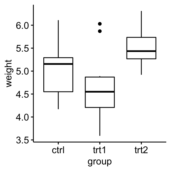
Check assumptions
Outliers
Outliers can be easily identified using box plot methods, implemented in the R function identify_outliers() [rstatix package].
PlantGrowth %>%
  group_by(group) %>%
  identify_outliers(weight)
## # A tibble: 2 x 4
## group weight is.outlier is.extreme
## <fct> <dbl> <lgl> <lgl>
## 1 trt1 5.87 TRUE FALSE
## 2 trt1 6.03 TRUE FALSEThere were no extreme outliers.
Note that, in the situation where you have extreme outliers, this can be due to: 1) data entry errors, measurement errors or unusual values.
Yo can include the outlier in the analysis anyway if you do not believe the result will be substantially affected. This can be evaluated by comparing the result of the ANOVA test with and without the outlier.
It’s also possible to keep the outliers in the data and perform robust ANOVA test using the WRS2 package.
Normality assumption
The normality assumption can be checked by using one of the following two approaches:
- Analyzing the ANOVA model residuals to check the normality for all groups together. This approach is easier and it’s very handy when you have many groups or if there are few data points per group.
- Check normality for each group separately. This approach might be used when you have only a few groups and many data points per group.
In this section, we’ll show you how to proceed for both option 1 and 2.
Check normality assumption by analyzing the model residuals. QQ plot and Shapiro-Wilk test of normality are used. QQ plot draws the correlation between a given data and the normal distribution.
# Build the linear model
model  <- lm(weight ~ group, data = PlantGrowth)
# Create a QQ plot of residuals
ggqqplot(residuals(model))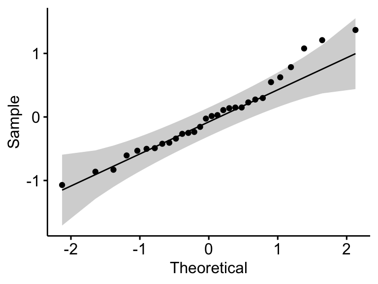
# Compute Shapiro-Wilk test of normality
shapiro_test(residuals(model))
## # A tibble: 1 x 3
## variable statistic p.value
## <chr> <dbl> <dbl>
## 1 residuals(model) 0.966 0.438In the QQ plot, as all the points fall approximately along the reference line, we can assume normality. This conclusion is supported by the Shapiro-Wilk test. The p-value is not significant (p = 0.13), so we can assume normality.
Check normality assumption by groups. Computing Shapiro-Wilk test for each group level. If the data is normally distributed, the p-value should be greater than 0.05.
PlantGrowth %>%
  group_by(group) %>%
  shapiro_test(weight)
## # A tibble: 3 x 4
## group variable statistic p
## <fct> <chr> <dbl> <dbl>
## 1 ctrl weight 0.957 0.747
## 2 trt1 weight 0.930 0.452
## 3 trt2 weight 0.941 0.564The score were normally distributed (p > 0.05) for each group, as assessed by Shapiro-Wilk’s test of normality.
Note that, if your sample size is greater than 50, the normal QQ plot is preferred because at larger sample sizes the Shapiro-Wilk test becomes very sensitive even to a minor deviation from normality.
QQ plot draws the correlation between a given data and the normal distribution. Create QQ plots for each group level:
ggqqplot(PlantGrowth, "weight", facet.by = "group")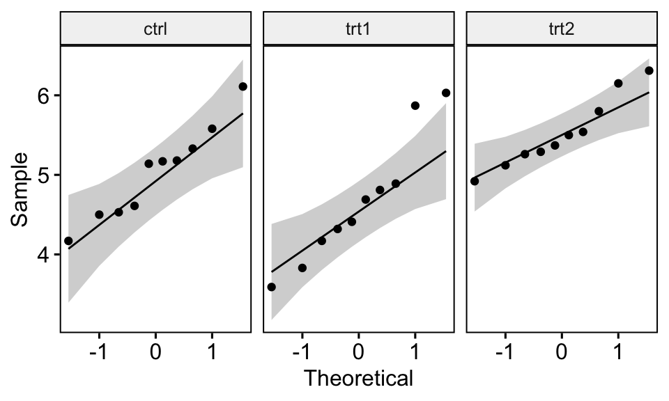
All the points fall approximately along the reference line, for each cell. So we can assume normality of the data.
If you have doubt about the normality of the data, you can use the Kruskal-Wallis test, which is the non-parametric alternative to one-way ANOVA test.
Homogneity of variance assumption
- The residuals versus fits plot can be used to check the homogeneity of variances.
plot(model, 1)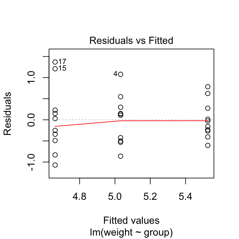
In the plot above, there is no evident relationships between residuals and fitted values (the mean of each groups), which is good. So, we can assume the homogeneity of variances.
- It’s also possible to use the Levene’s test to check the homogeneity of variances:
PlantGrowth %>% levene_test(weight ~ group)## # A tibble: 1 x 4
## df1 df2 statistic p
## <int> <int> <dbl> <dbl>
## 1 2 27 1.12 0.341From the output above, we can see that the p-value is > 0.05, which is not significant. This means that, there is not significant difference between variances across groups. Therefore, we can assume the homogeneity of variances in the different treatment groups.
In a situation where the homogeneity of variance assumption is not met, you can compute the Welch one-way ANOVA test using the function welch_anova_test()[rstatix package]. This test does not require the assumption of equal variances.
Computation
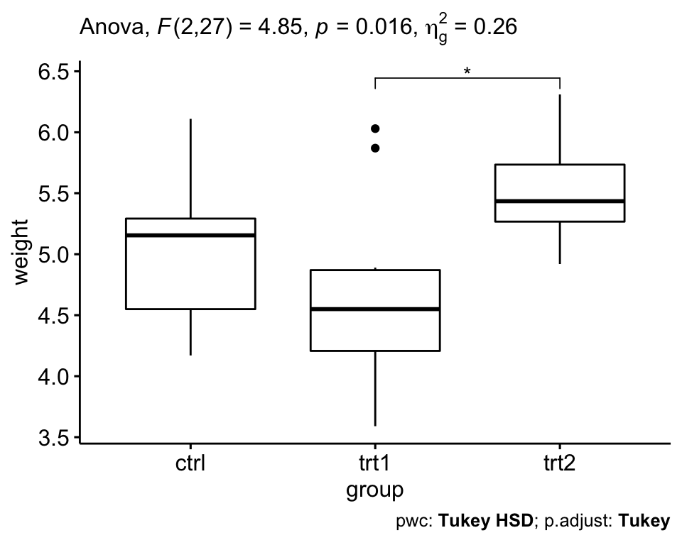
res.aov <- PlantGrowth %>% anova_test(weight ~ group)
res.aov
## ANOVA Table (type II tests)
##
## Effect DFn DFd F p p<.05 ges
## 1 group 2 27 4.85 0.016 * 0.264In the table above, the column ges corresponds to the generalized eta squared (effect size). It measures the proportion of the variability in the outcome variable (here plant weight) that can be explained in terms of the predictor (here, treatment group). An effect size of 0.26 (26%) means that 26% of the change in the weight can be accounted for the treatment conditions.
From the above ANOVA table, it can be seen that there are significant differences between groups (p = 0.016), which are highlighted with “*“, F(2, 27) = 4.85, p = 0.16, eta2[g] = 0.26.
where,
Findicates that we are comparing to an F-distribution (F-test);(2, 27)indicates the degrees of freedom in the numerator (DFn) and the denominator (DFd), respectively;4.85indicates the obtained F-statistic valuepspecifies the p-valuegesis the generalized effect size (amount of variability due to the factor)
Post-hoc tests
A significant one-way ANOVA is generally followed up by Tukey post-hoc tests to perform multiple pairwise comparisons between groups. Key R function: tukey_hsd() [rstatix].
# Pairwise comparisons
pwc <- PlantGrowth %>% tukey_hsd(weight ~ group)
pwc
## # A tibble: 3 x 8
## term group1 group2 estimate conf.low conf.high p.adj p.adj.signif
## * <chr> <chr> <chr> <dbl> <dbl> <dbl> <dbl> <chr>
## 1 group ctrl trt1 -0.371 -1.06 0.320 0.391 ns
## 2 group ctrl trt2 0.494 -0.197 1.19 0.198 ns
## 3 group trt1 trt2 0.865 0.174 1.56 0.012 *The output contains the following columns:
estimate: estimate of the difference between means of the two groupsconf.low,conf.high: the lower and the upper end point of the confidence interval at 95% (default)p.adj: p-value after adjustment for the multiple comparisons.
It can be seen from the output, that only the difference between trt2 and trt1 is significant (adjusted p-value = 0.012).
Report
We could report the results of one-way ANOVA as follow:
A one-way ANOVA was performed to evaluate if the plant growth was different for the 3 different treatment groups: ctr (n = 10), trt1 (n = 10) and trt2 (n = 10).
Data is presented as mean +/- standard deviation. Plant growth was statistically significantly different between different treatment groups, F(2, 27) = 4.85, p = 0.016, generalized eta squared = 0.26.
Plant growth decreased in trt1 group (4.66 +/- 0.79) compared to ctr group (5.03 +/- 0.58). It increased in trt2 group (5.53 +/- 0.44) compared to trt1 and ctr group.
Tukey post-hoc analyses revealed that the increase from trt1 to trt2 (0.87, 95% CI (0.17 to 1.56)) was statistically significant (p = 0.012), but no other group differences were statistically significant.
# Visualization: box plots with p-values
pwc <- pwc %>% add_xy_position(x = "group")
ggboxplot(PlantGrowth, x = "group", y = "weight") +
  stat_pvalue_manual(pwc, hide.ns = TRUE) +
  labs(
    subtitle = get_test_label(res.aov, detailed = TRUE),
    caption = get_pwc_label(pwc)
    )
Relaxing the homogeneity of variance assumption
The classical one-way ANOVA test requires an assumption of equal variances for all groups. In our example, the homogeneity of variance assumption turned out to be fine: the Levene test is not significant.
How do we save our ANOVA test, in a situation where the homogeneity of variance assumption is violated?
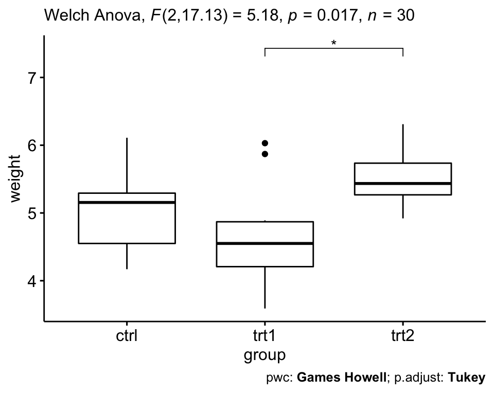
- The Welch one-way test is an alternative to the standard one-way ANOVA in the situation where the homogeneity of variance can’t be assumed (i.e., Levene test is significant).
- In this case, the Games-Howell post hoc test or pairwise t-tests (with no assumption of equal variances) can be used to compare all possible combinations of group differences.
# Welch One way ANOVA test
res.aov2 <- PlantGrowth %>% welch_anova_test(weight ~ group)
# Pairwise comparisons (Games-Howell)
pwc2 <- PlantGrowth %>% games_howell_test(weight ~ group)
# Visualization: box plots with p-values
pwc2 <- pwc2 %>% add_xy_position(x = "group", step.increase = 1)
ggboxplot(PlantGrowth, x = "group", y = "weight") +
  stat_pvalue_manual(pwc2, hide.ns = TRUE) +
  labs(
    subtitle = get_test_label(res.aov2, detailed = TRUE),
    caption = get_pwc_label(pwc2)
    )
You can also perform pairwise comparisons using pairwise t-test with no assumption of equal variances:
pwc3 <- PlantGrowth %>%
  pairwise_t_test(
    weight ~ group, pool.sd = FALSE,
    p.adjust.method = "bonferroni"
    )
pwc3
Two-way ANOVA
Data preparation
We’ll use the jobsatisfaction dataset [datarium package], which contains the job satisfaction score organized by gender and education levels.
In this study, a research wants to evaluate if there is a significant two-way interaction between gender and education_level on explaining the job satisfaction score. An interaction effect occurs when the effect of one independent variable on an outcome variable depends on the level of the other independent variables. If an interaction effect does not exist, main effects could be reported.
Load the data and inspect one random row by groups:
set.seed(123)
data("jobsatisfaction", package = "datarium")
jobsatisfaction %>% sample_n_by(gender, education_level, size = 1)
## # A tibble: 6 x 4
## id gender education_level score
## <fct> <fct> <fct> <dbl>
## 1 3 male school 5.07
## 2 17 male college 6.3
## 3 23 male university 10
## 4 37 female school 5.51
## 5 48 female college 5.65
## 6 49 female university 8.26In this example, the effect of “education_level” is our focal variable, that is our primary concern. It is thought that the effect of “education_level” will depend on one other factor, “gender”, which are called a moderator variable.
Summary statistics
Compute the mean and the SD (standard deviation) of the score by groups:
jobsatisfaction %>%
  group_by(gender, education_level) %>%
  get_summary_stats(score, type = "mean_sd")
## # A tibble: 6 x 6
## gender education_level variable n mean sd
## <fct> <fct> <chr> <dbl> <dbl> <dbl>
## 1 male school score 9 5.43 0.364
## 2 male college score 9 6.22 0.34
## 3 male university score 10 9.29 0.445
## 4 female school score 10 5.74 0.474
## 5 female college score 10 6.46 0.475
## 6 female university score 10 8.41 0.938Visualization
Create a box plot of the score by gender levels, colored by education levels:
bxp <- ggboxplot(
  jobsatisfaction, x = "gender", y = "score",
  color = "education_level", palette = "jco"
  )
bxp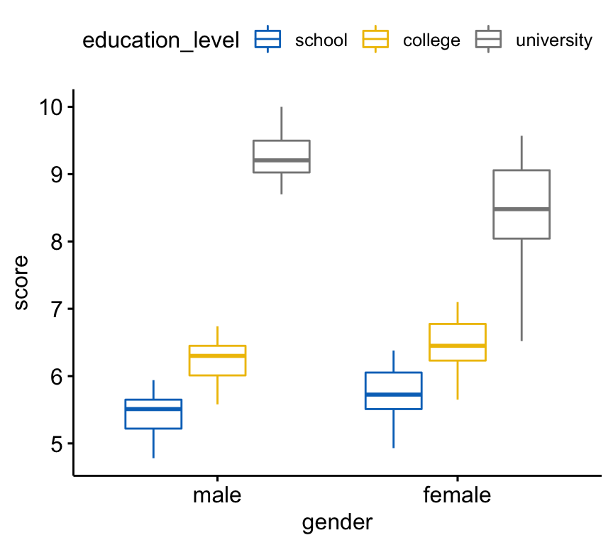
Check assumptions
Outliers
Identify outliers in each cell design:
jobsatisfaction %>%
  group_by(gender, education_level) %>%
  identify_outliers(score)
There were no extreme outliers.
Normality assumption
Check normality assumption by analyzing the model residuals. QQ plot and Shapiro-Wilk test of normality are used.
# Build the linear model
model  <- lm(score ~ gender*education_level,
             data = jobsatisfaction)
# Create a QQ plot of residuals
ggqqplot(residuals(model))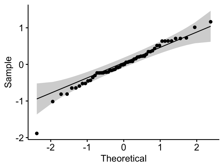
# Compute Shapiro-Wilk test of normality
shapiro_test(residuals(model))
## # A tibble: 1 x 3
## variable statistic p.value
## <chr> <dbl> <dbl>
## 1 residuals(model) 0.968 0.127In the QQ plot, as all the points fall approximately along the reference line, we can assume normality. This conclusion is supported by the Shapiro-Wilk test. The p-value is not significant (p = 0.13), so we can assume normality.
Check normality assumption by groups. Computing Shapiro-Wilk test for each combinations of factor levels:
jobsatisfaction %>%
  group_by(gender, education_level) %>%
  shapiro_test(score)
## # A tibble: 6 x 5
## gender education_level variable statistic p
## <fct> <fct> <chr> <dbl> <dbl>
## 1 male school score 0.980 0.966
## 2 male college score 0.958 0.779
## 3 male university score 0.916 0.323
## 4 female school score 0.963 0.819
## 5 female college score 0.963 0.819
## 6 female university score 0.950 0.674The score were normally distributed (p > 0.05) for each cell, as assessed by Shapiro-Wilk’s test of normality.
Create QQ plots for each cell of design:
ggqqplot(jobsatisfaction, "score", ggtheme = theme_bw()) +
  facet_grid(gender ~ education_level)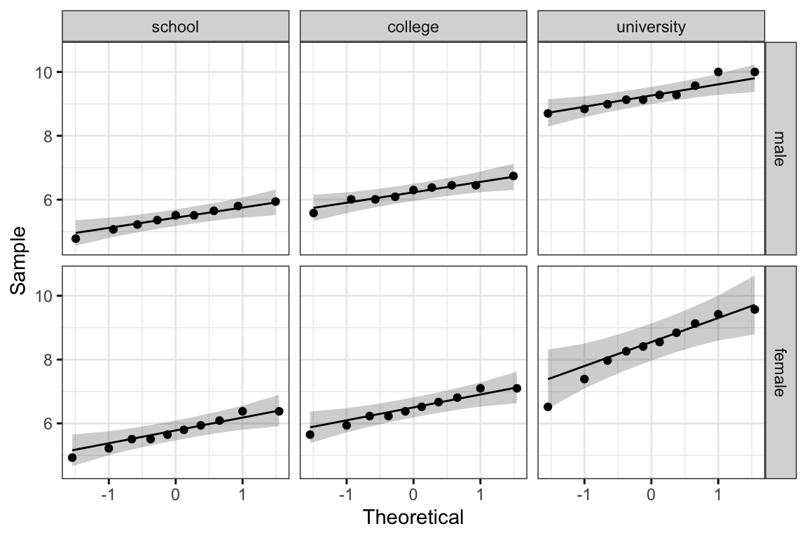
All the points fall approximately along the reference line, for each cell. So we can assume normality of the data.
Homogneity of variance assumption
This can be checked using the Levene’s test:
jobsatisfaction %>% levene_test(score ~ gender*education_level)## # A tibble: 1 x 4
## df1 df2 statistic p
## <int> <int> <dbl> <dbl>
## 1 5 52 2.20 0.0686The Levene’s test is not significant (p > 0.05). Therefore, we can assume the homogeneity of variances in the different groups.
Computation
In the R code below, the asterisk represents the interaction effect and the main effect of each variable (and all lower-order interactions).
res.aov <- jobsatisfaction %>% anova_test(score ~ gender * education_level)
res.aov
## ANOVA Table (type II tests)
##
## Effect DFn DFd F p p<.05 ges
## 1 gender 1 52 0.745 3.92e-01 0.014
## 2 education_level 2 52 187.892 1.60e-24 * 0.878
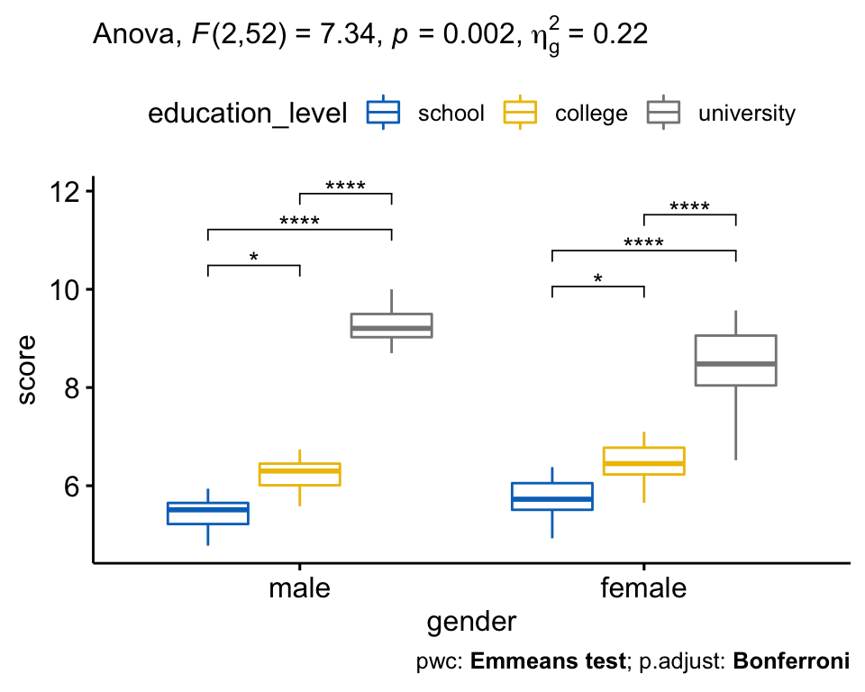
## 3 gender:education_level 2 52 7.338 2.00e-03 * 0.220There was a statistically significant interaction between gender and level of education for job satisfaction score, F(2, 52) = 7.34, p = 0.002.
Post-hoct tests
A significant two-way interaction indicates that the impact that one factor (e.g., education_level) has on the outcome variable (e.g., job satisfaction score) depends on the level of the other factor (e.g., gender) (and vice versa). So, you can decompose a significant two-way interaction into:
- Simple main effect: run one-way model of the first variable at each level of the second variable,
- Simple pairwise comparisons: if the simple main effect is significant, run multiple pairwise comparisons to determine which groups are different.
For a non-significant two-way interaction, you need to determine whether you have any statistically significant main effects from the ANOVA output. A significant main effect can be followed up by pairwise comparisons between groups.
Procedure for significant two-way interaction
Compute simple main effects
In our example, you could therefore investigate the effect of education_level at every level of gender or investigate the effect of gender at every level of the variable education_level.
Here, we’ll run a one-way ANOVA of education_level at each levels of gender.
Note that, if you have met the assumptions of the two-way ANOVA (e.g., homogeneity of variances), it is better to use the overall error term (from the two-way ANOVA) as input in the one-way ANOVA model. This will make it easier to detect any statistically significant differences if they exist (Keppel & Wickens, 2004; Maxwell & Delaney, 2004).
When you have failed the homogeneity of variances assumptions, you might consider running separate one-way ANOVAs with separate error terms.
In the R code below, we’ll group the data by gender and analyze the simple main effects of education level on Job Satisfaction score. The argument error is used to specify the ANOVA model from which the pooled error sum of squares and degrees of freedom are to be calculated.
# Group the data by gender and fit  anova
model <- lm(score ~ gender * education_level, data = jobsatisfaction)
jobsatisfaction %>%
  group_by(gender) %>%
  anova_test(score ~ education_level, error = model)
## # A tibble: 2 x 8
## gender Effect DFn DFd F p `p<.05` ges
## <fct> <chr> <dbl> <dbl> <dbl> <dbl> <chr> <dbl>
## 1 male education_level 2 52 132. 3.92e-21 * 0.836
## 2 female education_level 2 52 62.8 1.35e-14 * 0.707The simple main effect of “education_level” on job satisfaction score was statistically significant for both male and female (p < 0.0001).
In other words, there is a statistically significant difference in mean job satisfaction score between males educated to either school, college or university level, F(2, 52) = 132, p < 0.0001. The same conclusion holds true for females, F(2, 52) = 62.8, p < 0.0001.
Note that, statistical significance of the simple main effect analyses was accepted at a Bonferroni-adjusted alpha level of 0.025. This corresponds to the current level you declare statistical significance at (i.e., p < 0.05) divided by the number of simple main effect you are computing (i.e., 2).
Compute pairwise comparisons
A statistically significant simple main effect can be followed up by multiple pairwise comparisons to determine which group means are different. We’ll now perform multiple pairwise comparisons between the different education_level groups by gender.
You can run and interpret all possible pairwise comparisons using a Bonferroni adjustment. This can be easily done using the function emmeans_test() [rstatix package], a wrapper around the emmeans package, which needs to be installed. Emmeans stands for estimated marginal means (aka least square means or adjusted means).
Compare the score of the different education levels by gender levels:
# pairwise comparisons
library(emmeans)
pwc <- jobsatisfaction %>%
  group_by(gender) %>%
  emmeans_test(score ~ education_level, p.adjust.method = "bonferroni")
pwc
## # A tibble: 6 x 9
## gender .y. group1 group2 df statistic p p.adj p.adj.signif
## * <fct> <chr> <chr> <chr> <dbl> <dbl> <dbl> <dbl> <chr>
## 1 male score school college 52 -3.07 3.37e- 3 1.01e- 2 *
## 2 male score school university 52 -15.3 6.87e-21 2.06e-20 ****
## 3 male score college university 52 -12.1 8.42e-17 2.53e-16 ****
## 4 female score school college 52 -2.94 4.95e- 3 1.49e- 2 *
## 5 female score school university 52 -10.8 6.07e-15 1.82e-14 ****
## 6 female score college university 52 -7.90 1.84e-10 5.52e-10 ****There was a significant difference of job satisfaction score between all groups for both males and females (p < 0.05).
Procedure for non-significant two-way interaction
Inspect main effects
If the two-way interaction is not statistically significant, you need to consult the main effect for each of the two variables (gender and education_level) in the ANOVA output.
res.aov## ANOVA Table (type II tests)
##
## Effect DFn DFd F p p<.05 ges
## 1 gender 1 52 0.745 3.92e-01 0.014
## 2 education_level 2 52 187.892 1.60e-24 * 0.878
## 3 gender:education_level 2 52 7.338 2.00e-03 * 0.220In our example, there was a statistically significant main effects of education_level (F(2, 52) = 187.89, p < 0.0001) on the job satisfaction score. However, the main effect of gender was not significant, F (1, 52) = 0.74, p = 0.39.
Compute pairwise comparisons
Perform pairwise comparisons between education level groups to determine which groups are significantly different. Bonferroni adjustment is applied. This analysis can be done using simply the R base function pairwise_t_test() or using the function emmeans_test().
- Pairwise t-test:
jobsatisfaction %>%
  pairwise_t_test(
    score ~ education_level,
    p.adjust.method = "bonferroni"
    )
All pairwise differences were statistically significant (p < 0.05).
- Pairwise comparisons using Emmeans test. You need to specify the overall model, from which the overall degrees of freedom are to be calculated. This will make it easier to detect any statistically significant differences if they exist.
model <- lm(score ~ gender * education_level, data = jobsatisfaction)
jobsatisfaction %>%
  emmeans_test(
    score ~ education_level, p.adjust.method = "bonferroni",
    model = model
    )
Report
A two-way ANOVA was conducted to examine the effects of gender and education level on job satisfaction score.
Residual analysis was performed to test for the assumptions of the two-way ANOVA. Outliers were assessed by box plot method, normality was assessed using Shapiro-Wilk’s normality test and homogeneity of variances was assessed by Levene’s test.
There were no extreme outliers, residuals were normally distributed (p > 0.05) and there was homogeneity of variances (p > 0.05).
There was a statistically significant interaction between gender and education level on job satisfaction score, F(2, 52) = 7.33, p = 0.0016, eta2[g] = 0.22.
Consequently, an analysis of simple main effects for education level was performed with statistical significance receiving a Bonferroni adjustment. There was a statistically significant difference in mean “job satisfaction” scores for both males (F(2, 52) = 132, p < 0.0001) and females (F(2, 52) = 62.8, p < 0.0001) educated to either school, college or university level.
All pairwise comparisons were analyzed between the different education_level groups organized by gender. There was a significant difference of Job Satisfaction score between all groups for both males and females (p < 0.05).
# Visualization: box plots with p-values
pwc <- pwc %>% add_xy_position(x = "gender")
bxp +
  stat_pvalue_manual(pwc) +
  labs(
    subtitle = get_test_label(res.aov, detailed = TRUE),
    caption = get_pwc_label(pwc)
    )
Three-Way ANOVA
The three-way ANOVA is an extension of the two-way ANOVA for assessing whether there is an interaction effect between three independent categorical variables on a continuous outcome variable.
Data preparation
We’ll use the headache dataset [datarium package], which contains the measures of migraine headache episode pain score in 72 participants treated with three different treatments. The participants include 36 males and 36 females. Males and females were further subdivided into whether they were at low or high risk of migraine.
We want to understand how each independent variable (type of treatments, risk of migraine and gender) interact to predict the pain score.
Load the data and inspect one random row by group combinations:
set.seed(123)
data("headache", package = "datarium")
headache %>% sample_n_by(gender, risk, treatment, size = 1)
## # A tibble: 12 x 5
## id gender risk treatment pain_score
## <int> <fct> <fct> <fct> <dbl>
## 1 20 male high X 100
## 2 29 male high Y 91.2
## 3 33 male high Z 81.3
## 4 6 male low X 73.1
## 5 12 male low Y 67.9
## 6 13 male low Z 75.0
## # … with 6 more rowsIn this example, the effect of the treatment types is our focal variable, that is our primary concern. It is thought that the effect of treatments will depend on two other factors, “gender” and “risk” level of migraine, which are called moderator variables.
Summary statistics
Compute the mean and the standard deviation (SD) of pain_score by groups:
headache %>%
  group_by(gender, risk, treatment) %>%
  get_summary_stats(pain_score, type = "mean_sd")
## # A tibble: 12 x 7
## gender risk treatment variable n mean sd
## <fct> <fct> <fct> <chr> <dbl> <dbl> <dbl>
## 1 male high X pain_score 6 92.7 5.12
## 2 male high Y pain_score 6 82.3 5.00
## 3 male high Z pain_score 6 79.7 4.05
## 4 male low X pain_score 6 76.1 3.86
## 5 male low Y pain_score 6 73.1 4.76
## 6 male low Z pain_score 6 74.5 4.89
## # … with 6 more rowsVisualization
Create a box plot of pain_score by treatment, color lines by risk groups and facet the plot by gender:
bxp <- ggboxplot(
  headache, x = "treatment", y = "pain_score",
  color = "risk", palette = "jco", facet.by = "gender"
  )
bxp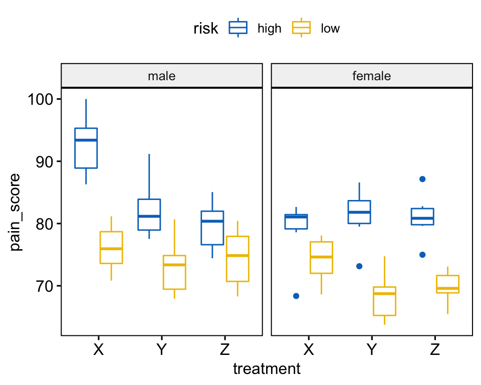
Check assumptions
Outliers
Identify outliers by groups:
headache %>%
  group_by(gender, risk, treatment) %>%
  identify_outliers(pain_score)
## # A tibble: 4 x 7
## gender risk treatment id pain_score is.outlier is.extreme
## <fct> <fct> <fct> <int> <dbl> <lgl> <lgl>
## 1 female high X 57 68.4 TRUE TRUE
## 2 female high Y 62 73.1 TRUE FALSE
## 3 female high Z 67 75.0 TRUE FALSE
## 4 female high Z 71 87.1 TRUE FALSEIt can be seen that, the data contain one extreme outlier (id = 57, female at high risk of migraine taking drug X)
Outliers can be due to: 1) data entry errors, 2) measurement errors or 3) unusual values.
Yo can include the outlier in the analysis anyway if you do not believe the result will be substantially affected. This can be evaluated by comparing the result of the ANOVA test with and without the outlier.
It’s also possible to keep the outliers in the data and perform robust ANOVA test using the WRS2 package.
Normality assumption
Check normality assumption by analyzing the model residuals. QQ plot and Shapiro-Wilk test of normality are used.
model  <- lm(pain_score ~ gender*risk*treatment, data = headache)
# Create a QQ plot of residuals
ggqqplot(residuals(model))
# Compute Shapiro-Wilk test of normality
shapiro_test(residuals(model))
## # A tibble: 1 x 3
## variable statistic p.value
## <chr> <dbl> <dbl>
## 1 residuals(model) 0.982 0.398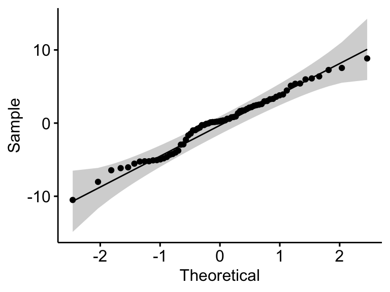
In the QQ plot, as all the points fall approximately along the reference line, we can assume normality. This conclusion is supported by the Shapiro-Wilk test. The p-value is not significant (p = 0.4), so we can assume normality.
Check normality assumption by groups. Computing Shapiro-Wilk test for each combinations of factor levels.
headache %>%
  group_by(gender, risk, treatment) %>%
  shapiro_test(pain_score)
## # A tibble: 12 x 6
## gender risk treatment variable statistic p
## <fct> <fct> <fct> <chr> <dbl> <dbl>
## 1 male high X pain_score 0.958 0.808
## 2 male high Y pain_score 0.902 0.384
## 3 male high Z pain_score 0.955 0.784
## 4 male low X pain_score 0.982 0.962
## 5 male low Y pain_score 0.920 0.507
## 6 male low Z pain_score 0.924 0.535
## # … with 6 more rowsThe pain scores were normally distributed (p > 0.05) except for one group (female at high risk of migraine taking drug X, p = 0.0086), as assessed by Shapiro-Wilk’s test of normality.
Create QQ plot for each cell of design:
ggqqplot(headache, "pain_score", ggtheme = theme_bw()) +
  facet_grid(gender + risk ~ treatment, labeller = "label_both")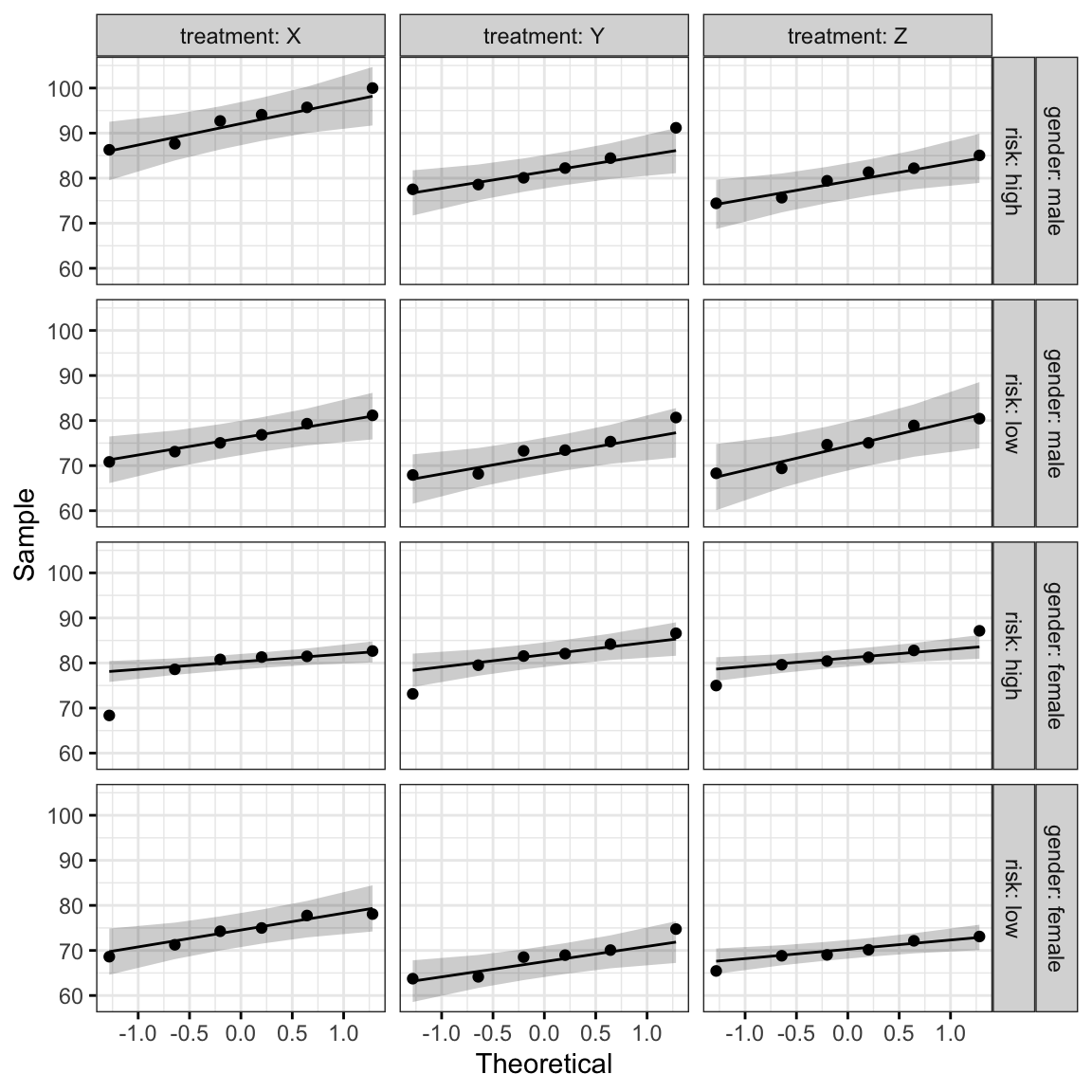
All the points fall approximately along the reference line, except for one group (female at high risk of migraine taking drug X), where we already identified an extreme outlier.
Homogneity of variance assumption
This can be checked using the Levene’s test:
headache %>% levene_test(pain_score ~ gender*risk*treatment)## # A tibble: 1 x 4
## df1 df2 statistic p
## <int> <int> <dbl> <dbl>
## 1 11 60 0.179 0.998The Levene’s test is not significant (p > 0.05). Therefore, we can assume the homogeneity of variances in the different groups.
Computation
res.aov <- headache %>% anova_test(pain_score ~ gender*risk*treatment)
res.aov
## ANOVA Table (type II tests)
##
## Effect DFn DFd F p p<.05 ges
## 1 gender 1 60 16.196 1.63e-04 * 0.213
## 2 risk 1 60 92.699 8.80e-14 * 0.607
## 3 treatment 2 60 7.318 1.00e-03 * 0.196
## 4 gender:risk 1 60 0.141 7.08e-01 0.002
## 5 gender:treatment 2 60 3.338 4.20e-02 * 0.100
## 6 risk:treatment 2 60 0.713 4.94e-01 0.023
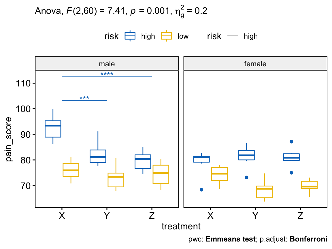
## 7 gender:risk:treatment 2 60 7.406 1.00e-03 * 0.198There was a statistically significant three-way interaction between gender, risk and treatment, F(2, 60) = 7.41, p = 0.001.
Post-hoc tests
If there is a significant three-way interaction effect, you can decompose it into:
- Simple two-way interaction: run two-way interaction at each level of third variable,
- Simple simple main effect: run one-way model at each level of second variable, and
- simple simple pairwise comparisons: run pairwise or other post-hoc comparisons if necessary.
If you do not have a statistically significant three-way interaction, you need to determine whether you have any statistically significant two-way interaction from the ANOVA output. You can follow up a significant two-way interaction by simple main effects analyses and pairwise comparisons between groups if necessary.
In this section we’ll describe the procedure for a significant three-way interaction.
Compute simple two-way interactions
You are free to decide which two variables will form the simple two-way interactions and which variable will act as the third (moderator) variable. In our example, we want to evaluate the effect of risk*treatment interaction on pain_score at each level of gender.
Note that, when doing the two-way interaction analysis, it’s better to use the overall error term (or residuals) from the three-way ANOVA result, obtained previously using the whole dataset. This is particularly recommended when the homogeneity of variance assumption is met (Keppel & Wickens, 2004).
The use of group-specific error term is “safer” from any violations of the assumptions. However, the pooled error terms have greater power – particularly with small sample sizes – but are susceptible to problems if there are any violations of assumptions.
In the R code below, we’ll group the data by gender and fit the treatment*risk two-way interaction. The argument error is used to specify the three-way ANOVA model from which the pooled error sum of squares and degrees of freedom are to be calculated.
# Group the data by gender and
# fit simple two-way interaction
model  <- lm(pain_score ~ gender*risk*treatment, data = headache)
headache %>%
  group_by(gender) %>%
  anova_test(pain_score ~ risk*treatment, error = model)
## # A tibble: 6 x 8
## gender Effect DFn DFd F p `p<.05` ges
## <fct> <chr> <dbl> <dbl> <dbl> <dbl> <chr> <dbl>
## 1 male risk 1 60 50.0 0.00000000187 * 0.455
## 2 male treatment 2 60 10.2 0.000157 * 0.253
## 3 male risk:treatment 2 60 5.25 0.008 * 0.149
## 4 female risk 1 60 42.8 0.0000000150 * 0.416
## 5 female treatment 2 60 0.482 0.62 "" 0.016
## 6 female risk:treatment 2 60 2.87 0.065 "" 0.087There was a statistically significant simple two-way interaction between risk and treatment (risk:treatment) for males, F(2, 60) = 5.25, p = 0.008, but not for females, F(2, 60) = 2.87, p = 0.065.
For males, this result suggests that the effect of treatment on “pain_score” depends on one’s “risk” of migraine. In other words, the risk moderates the effect of the type of treatment on pain_score.
Note that, statistical significance of a simple two-way interaction was accepted at a Bonferroni-adjusted alpha level of 0.025. This corresponds to the current level you declare statistical significance at (i.e., p < 0.05) divided by the number of simple two-way interaction you are computing (i.e., 2).
Compute simple simple main effects
A statistically significant simple two-way interaction can be followed up with simple simple main effects. In our example, you could therefore investigate the effect of treatment on pain_score at every level of risk or investigate the effect of risk at every level of treatment.
You will only need to do this for the simple two-way interaction for “males” as this was the only simple two-way interaction that was statistically significant. The error term again comes from the three-way ANOVA.
Group the data by gender and risk and analyze the simple simple main effects of treatment on pain_score:
# Group the data by gender and risk, and fit  anova
treatment.effect <- headache %>%
  group_by(gender, risk) %>%
  anova_test(pain_score ~ treatment, error = model)
treatment.effect %>% filter(gender == "male")
## # A tibble: 2 x 9
## gender risk Effect DFn DFd F p `p<.05` ges
## <fct> <fct> <chr> <dbl> <dbl> <dbl> <dbl> <chr> <dbl>
## 1 male high treatment 2 60 14.8 0.0000061 * 0.33
## 2 male low treatment 2 60 0.66 0.521 "" 0.022In the table above, we only need the results for the simple simple main effects of treatment for: (1) “males” at “low” risk; and (2) “males” at “high” risk.
Statistical significance was accepted at a Bonferroni-adjusted alpha level of 0.025, that is 0.05 divided y the number of simple simple main effects you are computing (i.e., 2).
There was a statistically significant simple simple main effect of treatment for males at high risk of migraine, F(2, 60) = 14.8, p < 0.0001), but not for males at low risk of migraine, F(2, 60) = 0.66, p = 0.521.
This analysis indicates that, the type of treatment taken has a statistically significant effect on pain_score in males who are at high risk.
In other words, the mean pain_score in the treatment X, Y and Z groups was statistically significantly different for males who at high risk, but not for males at low risk.
Compute simple simple comparisons
A statistically significant simple simple main effect can be followed up by multiple pairwise comparisons to determine which group means are different. This can be easily done using the function emmeans_test() [rstatix package] described in the previous section.
Compare the different treatments by gender and risk variables:
# Pairwise comparisons
library(emmeans)
pwc <- headache %>%
  group_by(gender, risk) %>%
  emmeans_test(pain_score ~ treatment, p.adjust.method = "bonferroni") %>%
  select(-df, -statistic, -p) # Remove details
# Show comparison results for male at high risk
pwc %>% filter(gender == "male", risk == "high")
## # A tibble: 3 x 7
## gender risk .y. group1 group2 p.adj p.adj.signif
## <fct> <fct> <chr> <chr> <chr> <dbl> <chr>
## 1 male high pain_score X Y 0.000386 ***
## 2 male high pain_score X Z 0.00000942 ****
## 3 male high pain_score Y Z 0.897 ns# Estimated marginal means (i.e. adjusted means)
# with 95% confidence interval
get_emmeans(pwc) %>% filter(gender == "male", risk == "high")## # A tibble: 3 x 9
## gender risk treatment emmean se df conf.low conf.high method
## <fct> <fct> <fct> <dbl> <dbl> <dbl> <dbl> <dbl> <chr>
## 1 male high X 92.7 1.80 60 89.1 96.3 Emmeans test
## 2 male high Y 82.3 1.80 60 78.7 85.9 Emmeans test
## 3 male high Z 79.7 1.80 60 76.1 83.3 Emmeans testIn the pairwise comparisons table above, we are interested only in the simple simple comparisons for males at a high risk of a migraine headache. In our example, there are three possible combinations of group differences.
For male at high risk, there was a statistically significant mean difference between treatment X and treatment Y of 10.4 (p.adj < 0.001), and between treatment X and treatment Z of 13.1 (p.adj < 0.0001).
However, the difference between treatment Y and treatment Z (2.66) was not statistically significant, p.adj = 0.897.
Report
A three-way ANOVA was conducted to determine the effects of gender, risk and treatment on migraine headache episode pain_score.
Residual analysis was performed to test for the assumptions of the three-way ANOVA. Normality was assessed using Shapiro-Wilk’s normality test and homogeneity of variances was assessed by Levene’s test.
Residuals were normally distributed (p > 0.05) and there was homogeneity of variances (p > 0.05).
There was a statistically significant three-way interaction between gender, risk and treatment, F(2, 60) = 7.41, p = 0.001.
Statistical significance was accepted at the p < 0.025 level for simple two-way interactions and simple simple main effects. There was a statistically significant simple two-way interaction between risk and treatment for males, F(2, 60) = 5.2, p = 0.008, but not for females, F(2, 60) = 2.8, p = 0.065.
There was a statistically significant simple simple main effect of treatment for males at high risk of migraine, F(2, 60) = 14.8, p < 0.0001), but not for males at low risk of migraine, F(2, 60) = 0.66, p = 0.521.
All simple simple pairwise comparisons, between the different treatment groups, were run for males at high risk of migraine with a Bonferroni adjustment applied.
There was a statistically significant mean difference between treatment X and treatment Y. However, the difference between treatment Y and treatment Z, was not statistically significant.
# Visualization: box plots with p-values
pwc <- pwc %>% add_xy_position(x = "treatment")
pwc.filtered <- pwc %>% filter(gender == "male", risk == "high")
bxp +
  stat_pvalue_manual(
    pwc.filtered, color = "risk", linetype = "risk", hide.ns = TRUE,
    tip.length = 0, step.increase = 0.1, step.group.by = "gender"
  ) +
  labs(
    subtitle = get_test_label(res.aov, detailed = TRUE),
    caption = get_pwc_label(pwc)
    )
Summary
This article describes how to compute and interpret ANOVA in R. We also explain the assumptions made by ANOVA tests and provide practical examples of R codes to check whether the test assumptions are met.
Recommended for you
This section contains best data science and self-development resources to help you on your path.
Books - Data Science
Our Books
- Practical Guide to Cluster Analysis in R by A. Kassambara (Datanovia)
- Practical Guide To Principal Component Methods in R by A. Kassambara (Datanovia)
- Machine Learning Essentials: Practical Guide in R by A. Kassambara (Datanovia)
- R Graphics Essentials for Great Data Visualization by A. Kassambara (Datanovia)
- GGPlot2 Essentials for Great Data Visualization in R by A. Kassambara (Datanovia)
- Network Analysis and Visualization in R by A. Kassambara (Datanovia)
- Practical Statistics in R for Comparing Groups: Numerical Variables by A. Kassambara (Datanovia)
- Inter-Rater Reliability Essentials: Practical Guide in R by A. Kassambara (Datanovia)
Others
- R for Data Science: Import, Tidy, Transform, Visualize, and Model Data by Hadley Wickham & Garrett Grolemund
- Hands-On Machine Learning with Scikit-Learn, Keras, and TensorFlow: Concepts, Tools, and Techniques to Build Intelligent Systems by Aurelien Géron
- Practical Statistics for Data Scientists: 50 Essential Concepts by Peter Bruce & Andrew Bruce
- Hands-On Programming with R: Write Your Own Functions And Simulations by Garrett Grolemund & Hadley Wickham
- An Introduction to Statistical Learning: with Applications in R by Gareth James et al.
- Deep Learning with R by François Chollet & J.J. Allaire
- Deep Learning with Python by François Chollet
Version:
 Français

First, I LOVE your site – it is incredibly informative and easy to follow. Thanks!!
I am trying to calculate the simple mean error as in the 2-way anova above, though I would like to do it for many variables at once, so I am trying to use the “map2” function of the purrr package. I have been unsuccessful and cannot figure out how to make this work.
Here is my data:
“` r
df # A tibble: 6 x 15
#> id edge trt nl lm md c mgg mgcm p sp ap
#>
#> 1 1 S C 1.80 -1.13 1.75 -0.303 2.94 1.02 1.60 1166. 1.10
#> 2 2 S T NA NA NA NA NA NA NA NA NA
#> 3 3 D C 1.60 -1.55 1.17 -0.341 1.85 0.787 1.41 663. 0.899
#> 4 4 D T 1.34 -2.22 0.962 -0.332 1.65 0.750 0.674 63.6 0.543
#> 5 5 S C 1.80 -0.165 2.16 -0.285 3.14 1.09 2.21 496. 1.16
#> 6 6 S T 2.14 0.250 2.44 -0.219 3.36 1.16 2.31 911. 1.20
#> # … with 3 more variables: la , lacm , lacmd
“`
I’ve successfully run all the two-way anovas I need:
“` r
models_1 %
group_by(edge) %>%
map2(ind.trans[4:15], models_1, ~ anova_test(.x, error = .y, type = 3))
#> Error in df %>% group_by(edge) %>% map2(ind.trans[4:15], models_1, ~anova_test(.x, : could not find function “%>%”
“`
I receive the following error, even though the number of columns I’m calling and the number of models match:
Error: Mapped vectors must have consistent lengths:
* `.x` has length 15
* `.y` has length 12
Thanks in advance!
Created on 2020-05-19 by the [reprex package](https://reprex.tidyverse.org) (v0.3.0)
Would you please provide a reproducible example as described at How to Include Reproducible R Script Examples in Datanovia Comments. You will need the pubr R package, which can be installed using devtools::install_github(“kassambara/pubr”)
Hi, About the post hoc test, I would like to know what is the difference between applying a pairwise.t.test and TukeyHSD test if I got a significant result from a Two Way ANOVA?
Thank you! It was very-very helpful!
I appreciate your positive feedback, thank you!
Hi, about your simple main effect and simple two-way interaction, you noted that it needs Bonferroni-adjusted p-value, yet I had noticed that many people do not do the adjustment. Does it necessary?
I like your site. It’s helpful! Thanks.
I am doing a three-way ANOVA, and I found that although you noted that it needs a Bonferroni-adjusted alpha level for simple two-way interaction and simple simple main effect in three-way ANOVA, many articles did not do the adjustment. I wonder if it is necessary to do the adjustment, or it’s ok if people don’t do it?
Hello, I have trouble adding the p-value of my post-Hoch test into a box plot. this message appears after running the code of the plot
Warning message:
Computation failed in `stat_bracket()`:
Internal error in `vec_proxy_assign_opts()`: `proxy` of type `double` incompatible with `value` proxy of type `integer`.
this is my code:
water <- read_xls("Water_cont2.xls")
str(water)

water <- as.data.frame(water)
water$treatment <- as.factor(water$treatment)
levels(water$treatment)


res.aov % anova_test(Water_Content ~ treatment)
res.aov

pwc % tukey_hsd(Water_Content ~ treatment)
pwc


pwc % add_xy_position(x = "treatment")
ggboxplot(water, x = "treatment", y = "Water_Content") +
  stat_pvalue_manual(pwc, hide.ns = TRUE) +
  labs(
    subtitle = get_test_label(res.aov, detailed = TRUE),
    caption = get_pwc_label(pwc)
  )
hope you can help me :)
thanks
Hi, you have some errors in your code. It should look like as follow:
Thank you for your help; however, the message is still appearing with your code.
Warning message:
Computation failed in `stat_bracket()`:
Internal error in `vec_proxy_assign_opts()`: `proxy` of type `double` incompatible with `value` proxy of type `integer`.
Does this error appears, when using the demo data in this tutorial? Would you please send your data, so that I can check?
Yes, it also happens with the demo data tutorial, so something must be wrong with my R. Should I download it again?
Probably the problem is with the operating system. I received the same message on a 64 bit system but the calculations were correct on a 32 bit system. Please check it at your place
Great that it works! The issue should be something related with your R sessions.
Hi,
First of all, thanks for the explanation. It’s very clear and easy to follow. I am concerned about the normality of the residuals assumption. I’m working with a 3×2 factorial design, with repeated measures in one of the two factors. In each of the six combinations, I have 8 -10 measures.
Do I have to check normality for each combination of factors or is it just one test with all the residuals?
Thanks very much.
Hello, thank you so much for this.
I have a simple question. What does “%>%” mean?
Thank you
In R,
%>%is the pipe operator. It takes the output of one statement and makes it the input of the next statement. When describing it, you can think of it as a “THEN”.Take, for example, the following code chunk:
The code chunk above will translate to something like “you take the Iris data, then you subset the data and then you print the data”.
I can’t get the following code to work:
headache %>%
group_by(gender, risk, treatment) %>%
shapiro_test(pain_score)
When I do this with my data I get an error:
Error: Problem with `mutate()` input `data`.
x Problem with `mutate()` input `data`.
x sample size must be between 3 and 5000
ℹ Input `data` is `map(.data$data, .f, …)`.
ℹ Input `data` is `map(.data$data, .f, …)`.
However, I can run the following format:
PlantGrowth %>%
group_by(group) %>%
shapiro_test(weight)
It appears that it is the group_by function that is failing. When I use either of my variables in the group_by() the shapiro_test() works. However, put together it always fails.
Any hints?
Also, I could imagine the work around: running the shapiro_test() two times, one for each variable.
e.g. Something like this twice, changing the group_by() variable each time.
PlantGrowth %>%
group_by(group) %>%
shapiro_test(weight)
Is that appropriate or will that ignore the influence of one variable on each test?
I also notice my other tibbles are shorter and appear to be only comparing the levels in one variable instead of two levels in both variables. Probably a related problem.
Any hints?
Dear Alboukadel Kassambara,
Thanks a lot for your great job, this tutorial about ANOVA is the best i ever seen, and i can’t stop using your R packages.
I have a question for you or anybody in this kind community : In my data set, i’m doing a 3-way anova, and then pairwise comparison, with bonferroni correction. My concern is about the N chosen by the algorithm to compute the correction. I have a lot of subset (4x3x5), and even if my df is about 100 rows, I think that my pwc (and so my bonferroni correction) should be computed only in each subset (about 5 rows) indepandantly. PWC are OK because of the use of the “group_by” function, but the BF corr. use the overall N instead of the N of the subset (leading to adjusted p-values divided by 100 in spite of 4-5). Am i wrong in my interpretation of the bonferroni correction ? If the idea seems right, does anybody have an idea on how to resolve that ? (i mean, not strictly manually dividing myself all p-values, recreating p.signif symbols, etc).
Thanks a lot to everybody !
Gaetan.
Dear Mr. Kassambara,
thank you so much for this amazing tutorial! It is the best I ever worked through, made so many things much clearer for me now and really helped me out with my thesis about animal movement data.
Kind regards
Thank you for your detailed descriptions. I have a question about how to switch the comparisons. For example, in the two-way ANOVA example, how would you write the model to compare gender at each education_level? Instead of comparing education_level of each gender as in the example.
Hi, thanks for the example. I am trying a 3-way anova. But experiencing with the codes.
This command is gicving me an error, and this not able to generate the anova table
treatment.effect %
group_by(gender, risk) %>%
anova_test(pain_score ~ treatment, error = model)
treatment.effect %>% filter(gender == “male”)
Error: Input must be a vector, not a object.
Backtrace:
1. treatment.effect %>% filter(gender == “male”)
11. vctrs:::stop_scalar_type(…)
12. vctrs:::stop_vctrs(msg, “vctrs_error_scalar_type”, actual = x)
Does anyone know how I can fix that?
Thks
Hi, thanks for a very helpful article. I have a question.
When I run the code for three-way anova, the simple-simple main effects with this script:
treatment.effect %
group_by(gender, risk) %>%
anova_test(pain_score ~ treatment, error = model)
treatment.effect %>% filter(gender == “male”)
It always shows this error notification
Error: Input must be a vector, not a object.
Do you know how to fix it?
Hello,
Everything worked so fine until the end with the final plot. The simple bxp is the same as showed but when I add the:
The simple bxp plots males first then female but after adding the stat_pvalue_manual() and labs() is inverted and pvalue lines are misplaced.
Can anyone explain why I get this error message when I run emmeans-test ;
Error in contrast.emmGrid(res.emmeans, by = grouping.vars, method = method, : Nonconforming number of contrast coefficients
Do we not need to check if the data is balanced?
Dear Alboukadel Kassambara,
I have a question, as we do Levene test when the assumption of normality doesn’t meet but in two way ANOVA the normality assumption is getting met in your results, if am not wrong you should have done the Bartlett test and according to the Bartlett p-value comes 0.02 which means it’s violating the assumption of homogeneity but Levene shows 0.06 value which means it meets the assumption, I’m a little bit confused why did you use Levene instead of Bartlett please clarify it.
Thanks
Thank you so much for providing very easy-to-follow stats in R