The repeated-measures ANOVA is used for analyzing data where same subjects are measured more than once. This test is also referred to as a within-subjects ANOVA or ANOVA with repeated measures. The “within-subjects” term means that the same individuals are measured on the same outcome variable under different time points or conditions.
For example, you might have measured 10 individuals’ self-esteem score (the outcome or dependent variable) on three time points during a specific diet to determine whether their self-esteem improved.
This chapter describes the different types of repeated measures ANOVA, including:
- One-way repeated measures ANOVA, an extension of the paired-samples t-test for comparing the means of three or more levels of a within-subjects variable.
- two-way repeated measures ANOVA used to evaluate simultaneously the effect of two within-subject factors on a continuous outcome variable.
- three-way repeated measures ANOVA used to evaluate simultaneously the effect of three within-subject factors on a continuous outcome variable.
The main goal of two-way and three-way repeated measures ANOVA is, respectively, to evaluate if there is a statistically significant interaction effect between two and three within-subjects factors in explaining a continuous outcome variable.
You will learn how to:
- Compute and interpret the different repeated measures ANOVA in R.
- Check repeated measures ANOVA test assumptions
- Perform post-hoc tests, multiple pairwise comparisons between groups to identify which groups are different
- Visualize the data using box plots, add ANOVA and pairwise comparisons p-values to the plot
Contents:
Related Book
Practical Statistics in R II - Comparing Groups: Numerical VariablesAssumptions
The repeated measures ANOVA makes the following assumptions about the data:
- No significant outliers in any cell of the design. This can be checked by visualizing the data using box plot methods and by using the function
identify_outliers()[rstatix package]. - Normality: the outcome (or dependent) variable should be approximately normally distributed in each cell of the design. This can be checked using the Shapiro-Wilk normality test (
shapiro_test()[rstatix]) or by visual inspection using QQ plot (ggqqplot()[ggpubr package]). - Assumption of sphericity: the variance of the differences between groups should be equal. This can be checked using the Mauchly’s test of sphericity, which is automatically reported when using the R function
anova_test()[rstatix package]. Read more in Chapter @ref(mauchly-s-test-of-sphericity-in-r).
Before computing repeated measures ANOVA test, you need to perform some preliminary tests to check if the assumptions are met.
Note that, if the above assumptions are not met there are a non-parametric alternative (Friedman test) to the one-way repeated measures ANOVA.
Unfortunately, there are no non-parametric alternatives to the two-way and the three-way repeated measures ANOVA. Thus, in the situation where the assumptions are not met, you could consider running the two-way/three-way repeated measures ANOVA on the transformed and non-transformed data to see if there are any meaningful differences.
If both tests lead you to the same conclusions, you might not choose to transform the outcome variable and carry on with the two-way/three-way repeated measures ANOVA on the original data.
It’s also possible to perform robust ANOVA test using the WRS2 R package.
No matter your choice, you should report what you did in your results.
Prerequisites
Make sure that you have installed the following R packages:
tidyversefor data manipulation and visualizationggpubrfor creating easily publication ready plotsrstatixprovides pipe-friendly R functions for easy statistical analysesdatarium: contains required data sets for this chapter
Start by loading the following R packages:
library(tidyverse)
library(ggpubr)
library(rstatix)
Key R functions:
anova_test()[rstatix package], a wrapper aroundcar::Anova()for making easy the computation of repeated measures ANOVA. Key arguments for performing repeated measures ANOVA:data: data framedv: (numeric) the dependent (or outcome) variable name.wid: variable name specifying the case/sample identifier.within: within-subjects factor or grouping variable
get_anova_table()[rstatix package]. Extracts the ANOVA table from the output ofanova_test(). It returns ANOVA table that is automatically corrected for eventual deviation from the sphericity assumption. The default is to apply automatically the Greenhouse-Geisser sphericity correction to only within-subject factors violating the sphericity assumption (i.e., Mauchly’s test p-value is significant, p <= 0.05). Read more in Chapter @ref(mauchly-s-test-of-sphericity-in-r).
One-way repeated measures ANOVA
Data preparation
We’ll use the self-esteem score dataset measured over three time points. The data is available in the datarium package.
# Data preparation
# Wide format
data("selfesteem", package = "datarium")
head(selfesteem, 3)
## # A tibble: 3 x 4
## id t1 t2 t3
## <int> <dbl> <dbl> <dbl>
## 1 1 4.01 5.18 7.11
## 2 2 2.56 6.91 6.31
## 3 3 3.24 4.44 9.78# Gather columns t1, t2 and t3 into long format
# Convert id and time into factor variables
selfesteem <- selfesteem %>%
gather(key = "time", value = "score", t1, t2, t3) %>%
convert_as_factor(id, time)
head(selfesteem, 3)## # A tibble: 3 x 3
## id time score
## <fct> <fct> <dbl>
## 1 1 t1 4.01
## 2 2 t1 2.56
## 3 3 t1 3.24The one-way repeated measures ANOVA can be used to determine whether the means self-esteem scores are significantly different between the three time points.
Summary statistics
Compute some summary statistics of the self-esteem score by groups (time): mean and sd (standard deviation)
selfesteem %>%
  group_by(time) %>%
  get_summary_stats(score, type = "mean_sd")
## # A tibble: 3 x 5
## time variable n mean sd
## <fct> <chr> <dbl> <dbl> <dbl>
## 1 t1 score 10 3.14 0.552
## 2 t2 score 10 4.93 0.863
## 3 t3 score 10 7.64 1.14Visualization
Create a box plot and add points corresponding to individual values:
bxp <- ggboxplot(selfesteem, x = "time", y = "score", add = "point")
bxp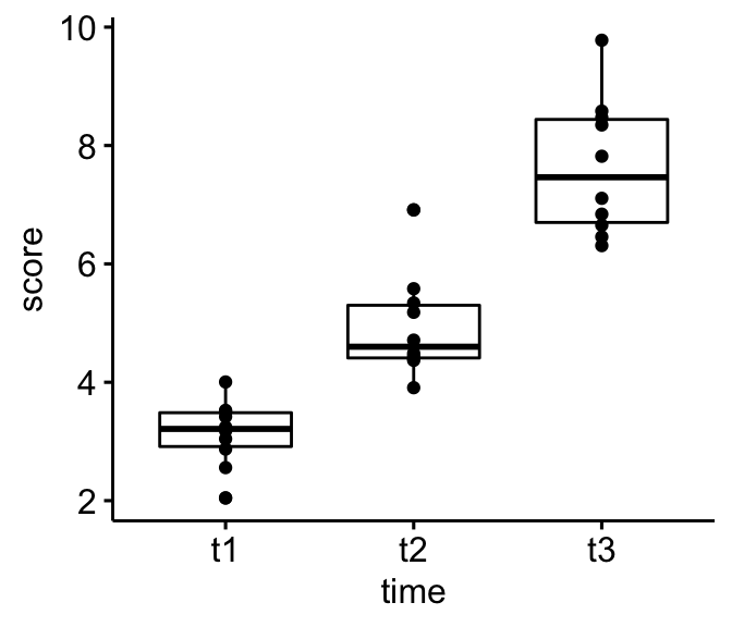
Check assumptions
Outliers
Outliers can be easily identified using box plot methods, implemented in the R function identify_outliers() [rstatix package].
selfesteem %>%
  group_by(time) %>%
  identify_outliers(score)
## # A tibble: 2 x 5
## time id score is.outlier is.extreme
## <fct> <fct> <dbl> <lgl> <lgl>
## 1 t1 6 2.05 TRUE FALSE
## 2 t2 2 6.91 TRUE FALSEThere were no extreme outliers.
Note that, in the situation where you have extreme outliers, this can be due to: 1) data entry errors, measurement errors or unusual values.
You can include the outlier in the analysis anyway if you do not believe the result will be substantially affected. This can be evaluated by comparing the result of the ANOVA with and without the outlier.
It’s also possible to keep the outliers in the data and perform robust ANOVA test using the WRS2 package.
Normality assumption
The normality assumption can be checked by computing Shapiro-Wilk test for each time point. If the data is normally distributed, the p-value should be greater than 0.05.
selfesteem %>%
  group_by(time) %>%
  shapiro_test(score)
## # A tibble: 3 x 4
## time variable statistic p
## <fct> <chr> <dbl> <dbl>
## 1 t1 score 0.967 0.859
## 2 t2 score 0.876 0.117
## 3 t3 score 0.923 0.380The self-esteem score was normally distributed at each time point, as assessed by Shapiro-Wilk’s test (p > 0.05).
Note that, if your sample size is greater than 50, the normal QQ plot is preferred because at larger sample sizes the Shapiro-Wilk test becomes very sensitive even to a minor deviation from normality.
QQ plot draws the correlation between a given data and the normal distribution. Create QQ plots for each time point:
ggqqplot(selfesteem, "score", facet.by = "time")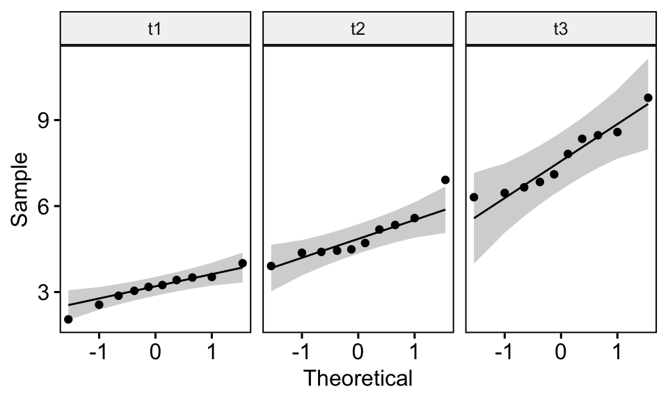
From the plot above, as all the points fall approximately along the reference line, we can assume normality.
Assumption of sphericity
As mentioned in previous sections, the assumption of sphericity will be automatically checked during the computation of the ANOVA test using the R function anova_test() [rstatix package]. The Mauchly’s test is internally used to assess the sphericity assumption.
By using the function get_anova_table() [rstatix] to extract the ANOVA table, the Greenhouse-Geisser sphericity correction is automatically applied to factors violating the sphericity assumption.
Computation
res.aov <- anova_test(data = selfesteem, dv = score, wid = id, within = time)
get_anova_table(res.aov)
## ANOVA Table (type III tests)
##
## Effect DFn DFd F p p<.05 ges
## 1 time 2 18 55.5 2.01e-08 * 0.829The self-esteem score was statistically significantly different at the different time points during the diet, F(2, 18) = 55.5, p < 0.0001, eta2[g] = 0.83.
where,
FIndicates that we are comparing to an F-distribution (F-test);(2, 18)indicates the degrees of freedom in the numerator (DFn) and the denominator (DFd), respectively;55.5indicates the obtained F-statistic valuepspecifies the p-valuegesis the generalized effect size (amount of variability due to the within-subjects factor)
Post-hoc tests
You can perform multiple pairwise paired t-tests between the levels of the within-subjects factor (here time). P-values are adjusted using the Bonferroni multiple testing correction method.
# pairwise comparisons
pwc <- selfesteem %>%
  pairwise_t_test(
    score ~ time, paired = TRUE,
    p.adjust.method = "bonferroni"
    )
pwc
## # A tibble: 3 x 10
## .y. group1 group2 n1 n2 statistic df p p.adj p.adj.signif
## * <chr> <chr> <chr> <int> <int> <dbl> <dbl> <dbl> <dbl> <chr>
## 1 score t1 t2 10 10 -4.97 9 0.000772 0.002 **
## 2 score t1 t3 10 10 -13.2 9 0.000000334 0.000001 ****
## 3 score t2 t3 10 10 -4.87 9 0.000886 0.003 **All the pairwise differences are statistically significant.
Report
We could report the result as follow:
The self-esteem score was statistically significantly different at the different time points, F(2, 18) = 55.5, p < 0.0001, generalized eta squared = 0.82.
Post-hoc analyses with a Bonferroni adjustment revealed that all the pairwise differences, between time points, were statistically significantly different (p <= 0.05).
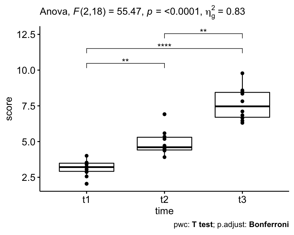
# Visualization: box plots with p-values
pwc <- pwc %>% add_xy_position(x = "time")
bxp +
  stat_pvalue_manual(pwc) +
  labs(
    subtitle = get_test_label(res.aov, detailed = TRUE),
    caption = get_pwc_label(pwc)
  )
Two-way repeated measures ANOVA
Data preparation
We’ll use the selfesteem2 dataset [in datarium package] containing the self-esteem score measures of 12 individuals enrolled in 2 successive short-term trials (4 weeks): control (placebo) and special diet trials.
Each participant performed all two trials. The order of the trials was counterbalanced and sufficient time was allowed between trials to allow any effects of previous trials to have dissipated.
The self-esteem score was recorded at three time points: at the beginning (t1), midway (t2) and at the end (t3) of the trials.
The question is to investigate if this short-term diet treatment can induce a significant increase of self-esteem score over time. In other terms, we wish to know if there is significant interaction between diet and time on the self-esteem score.
The two-way repeated measures ANOVA can be performed in order to determine whether there is a significant interaction between diet and time on the self-esteem score.
Load and show one random row by treatment group:
# Wide format
set.seed(123)
data("selfesteem2", package = "datarium")
selfesteem2 %>% sample_n_by(treatment, size = 1)
## # A tibble: 2 x 5
## id treatment t1 t2 t3
## <fct> <fct> <dbl> <dbl> <dbl>
## 1 4 ctr 92 92 89
## 2 10 Diet 90 93 95# Gather the columns t1, t2 and t3 into long format.
# Convert id and time into factor variables
selfesteem2 <- selfesteem2 %>%
gather(key = "time", value = "score", t1, t2, t3) %>%
convert_as_factor(id, time)
# Inspect some random rows of the data by groups
set.seed(123)
selfesteem2 %>% sample_n_by(treatment, time, size = 1)## # A tibble: 6 x 4
## id treatment time score
## <fct> <fct> <fct> <dbl>
## 1 4 ctr t1 92
## 2 10 ctr t2 84
## 3 5 ctr t3 68
## 4 11 Diet t1 93
## 5 12 Diet t2 80
## 6 1 Diet t3 88In this example, the effect of “time” on self-esteem score is our focal variable, that is our primary concern.
However, it is thought that the effect “time” will be different if treatment is performed or not. In this setting, the “treatment” variable is considered as moderator variable.
Summary statistics
Group the data by treatment and time, and then compute some summary statistics of the score variable: mean and sd (standard deviation).
selfesteem2 %>%
  group_by(treatment, time) %>%
  get_summary_stats(score, type = "mean_sd")
## # A tibble: 6 x 6
## treatment time variable n mean sd
## <fct> <fct> <chr> <dbl> <dbl> <dbl>
## 1 ctr t1 score 12 88 8.08
## 2 ctr t2 score 12 83.8 10.2
## 3 ctr t3 score 12 78.7 10.5
## 4 Diet t1 score 12 87.6 7.62
## 5 Diet t2 score 12 87.8 7.42
## 6 Diet t3 score 12 87.7 8.14Visualization
Create box plots of the score colored by treatment groups:
bxp <- ggboxplot(
  selfesteem2, x = "time", y = "score",
  color = "treatment", palette = "jco"
  )
bxp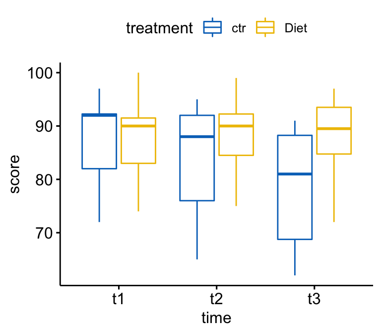
Chek assumptions
Outliers
selfesteem2 %>%
  group_by(treatment, time) %>%
  identify_outliers(score)
## [1] treatment time id score is.outlier is.extreme
## <0 rows> (or 0-length row.names)There were no extreme outliers.
Normality assumption
Compute Shapiro-Wilk test for each combinations of factor levels:
selfesteem2 %>%
  group_by(treatment, time) %>%
  shapiro_test(score)
## # A tibble: 6 x 5
## treatment time variable statistic p
## <fct> <fct> <chr> <dbl> <dbl>
## 1 ctr t1 score 0.828 0.0200
## 2 ctr t2 score 0.868 0.0618
## 3 ctr t3 score 0.887 0.107
## 4 Diet t1 score 0.919 0.279
## 5 Diet t2 score 0.923 0.316
## 6 Diet t3 score 0.886 0.104The self-esteem score was normally distributed at each time point (p > 0.05), except for ctr treatment at t1, as assessed by Shapiro-Wilk’s test.
Create QQ plot for each cell of design:
ggqqplot(selfesteem2, "score", ggtheme = theme_bw()) +
  facet_grid(time ~ treatment, labeller = "label_both")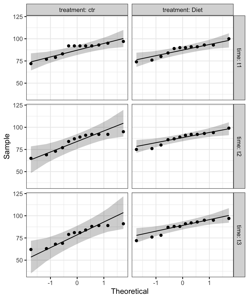
From the plot above, as all the points fall approximately along the reference line, we can assume normality.
Computation
res.aov <- anova_test(
  data = selfesteem2, dv = score, wid = id,
  within = c(treatment, time)
  )
get_anova_table(res.aov)
## ANOVA Table (type III tests)
##
## Effect DFn DFd F p p<.05 ges
## 1 treatment 1.00 11.0 15.5 2.00e-03 * 0.059
## 2 time 1.31 14.4 27.4 5.03e-05 * 0.049
## 3 treatment:time 2.00 22.0 30.4 4.63e-07 * 0.050There is a statistically significant two-way interactions between treatment and time, F(2, 22) = 30.4, p < 0.0001.
Post-hoc tests
A significant two-way interaction indicates that the impact that one factor (e.g., treatment) has on the outcome variable (e.g., self-esteem score) depends on the level of the other factor (e.g., time) (and vice versa). So, you can decompose a significant two-way interaction into:
- Simple main effect: run one-way model of the first variable (factor A) at each level of the second variable (factor B),
- Simple pairwise comparisons: if the simple main effect is significant, run multiple pairwise comparisons to determine which groups are different.
For a non-significant two-way interaction, you need to determine whether you have any statistically significant main effects from the ANOVA output.
Procedure for a significant two-way interaction
Effect of treatment. In our example, we’ll analyze the effect of treatment on self-esteem score at every time point.
Note that, the treatment factor variable has only two levels (“ctr” and “Diet”); thus, ANOVA test and paired t-test will give the same p-values.
# Effect of treatment at each time point
one.way <- selfesteem2 %>%
  group_by(time) %>%
  anova_test(dv = score, wid = id, within = treatment) %>%
  get_anova_table() %>%
  adjust_pvalue(method = "bonferroni")
one.way
## # A tibble: 3 x 9
## time Effect DFn DFd F p `p<.05` ges p.adj
## <fct> <chr> <dbl> <dbl> <dbl> <dbl> <chr> <dbl> <dbl>
## 1 t1 treatment 1 11 0.376 0.552 "" 0.000767 1
## 2 t2 treatment 1 11 9.03 0.012 * 0.052 0.036
## 3 t3 treatment 1 11 30.9 0.00017 * 0.199 0.00051# Pairwise comparisons between treatment groups
pwc <- selfesteem2 %>%
group_by(time) %>%
pairwise_t_test(
score ~ treatment, paired = TRUE,
p.adjust.method = "bonferroni"
)
pwc## # A tibble: 3 x 11
## time .y. group1 group2 n1 n2 statistic df p p.adj p.adj.signif
## * <fct> <chr> <chr> <chr> <int> <int> <dbl> <dbl> <dbl> <dbl> <chr>
## 1 t1 score ctr Diet 12 12 0.613 11 0.552 0.552 ns
## 2 t2 score ctr Diet 12 12 -3.00 11 0.012 0.012 *
## 3 t3 score ctr Diet 12 12 -5.56 11 0.00017 0.00017 ***Considering the Bonferroni adjusted p-value (p.adj), it can be seen that the simple main effect of treatment was not significant at the time point t1 (p = 1). It becomes significant at t2 (p = 0.036) and t3 (p = 0.00051).
Pairwise comparisons show that the mean self-esteem score was significantly different between ctr and Diet group at t2 (p = 0.12) and t3 (p = 0.00017) but not at t1 (p = 0.55).
Effect of time. Note that, it’s also possible to perform the same analysis for the time variable at each level of treatment. You don’t necessarily need to do this analysis.
The R code:
# Effect of time at each level of treatment
one.way2 <- selfesteem2 %>%
  group_by(treatment) %>%
  anova_test(dv = score, wid = id, within = time) %>%
  get_anova_table() %>%
  adjust_pvalue(method = "bonferroni")
# Pairwise comparisons between time points
pwc2 <- selfesteem2 %>%
  group_by(treatment) %>%
  pairwise_t_test(
    score ~ time, paired = TRUE,
    p.adjust.method = "bonferroni"
    )
pwc2
After executing the R code above, you can see that the effect of time is significant only for the control trial, F(2, 22) = 39.7, p < 0.0001. Pairwise comparisons show that all comparisons between time points were statistically significant for control trial.
Procedure for non-significant two-way interaction
If the interaction is not significant, you need to interpret the main effects for each of the two variables: treatment and time. A significant main effect can be followed up with pairwise comparisons.
In our example (see ANOVA table in res.aov), there was a statistically significant main effects of treatment (F(1, 11) = 15.5, p = 0.002) and time (F(2, 22) = 27.4, p < 0.0001) on the self-esteem score.
Pairwise paired t-test comparisons:
# comparisons for treatment variable
selfesteem2 %>%
  pairwise_t_test(
    score ~ treatment, paired = TRUE,
    p.adjust.method = "bonferroni"
    )
# comparisons for time variable
selfesteem2 %>%
  pairwise_t_test(
    score ~ time, paired = TRUE,
    p.adjust.method = "bonferroni"
    )
All pairwise comparisons are significant.
Report
We could report the result as follow:
A two-way repeated measures ANOVA was performed to evaluate the effect of different diet treatments over time on self-esteem score.
There was a statistically significant interaction between treatment and time on self-esteem score, F(2, 22) = 30.4, p < 0.0001. Therefore, the effect of treatment variable was analyzed at each time point. P-values were adjusted using the Bonferroni multiple testing correction method. The effect of treatment was significant at t2 (p = 0.036) and t3 (p = 0.00051) but not at the time point t1 (p = 1).
Pairwise comparisons, using paired t-test, show that the mean self-esteem score was significantly different between ctr and Diet trial at time points t2 (p = 0.012) and t3 (p = 0.00017) but not at t1 (p = 0.55).
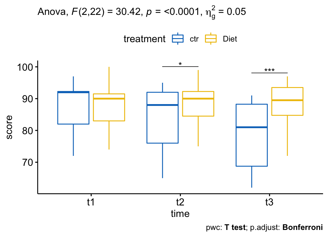
# Visualization: box plots with p-values
pwc <- pwc %>% add_xy_position(x = "time")
bxp +
  stat_pvalue_manual(pwc, tip.length = 0, hide.ns = TRUE) +
  labs(
    subtitle = get_test_label(res.aov, detailed = TRUE),
    caption = get_pwc_label(pwc)
  )
Three-way repeated measures ANOVA
Data preparation
We’ll use the weightloss dataset [datarium package]. In this study, a researcher wanted to assess the effects of Diet and Exercises on weight loss in 10 sedentary individuals.
The participants were enrolled in four trials: (1) no diet and no exercises; (2) diet only; (3) exercises only; and (4) diet and exercises combined.
Each participant performed all four trials. The order of the trials was counterbalanced and sufficient time was allowed between trials to allow any effects of previous trials to have dissipated.
Each trial lasted nine weeks and the weight loss score was measured at the beginning (t1), at the midpoint (t2) and at the end (t3) of each trial.
Three-way repeated measures ANOVA can be performed in order to determine whether there is a significant interaction between diet, exercises and time on the weight loss score.
Load the data and show some random rows by groups:
# Wide format
set.seed(123)
data("weightloss", package = "datarium")
weightloss %>% sample_n_by(diet, exercises, size = 1)
## # A tibble: 4 x 6
## id diet exercises t1 t2 t3
## <fct> <fct> <fct> <dbl> <dbl> <dbl>
## 1 4 no no 11.1 9.5 11.1
## 2 10 no yes 10.2 11.8 17.4
## 3 5 yes no 11.6 13.4 13.9
## 4 11 yes yes 12.7 12.7 15.1# Gather the columns t1, t2 and t3 into long format.
# Convert id and time into factor variables
weightloss <- weightloss %>%
gather(key = "time", value = "score", t1, t2, t3) %>%
convert_as_factor(id, time)
# Inspect some random rows of the data by groups
set.seed(123)
weightloss %>% sample_n_by(diet, exercises, time, size = 1)## # A tibble: 12 x 5
## id diet exercises time score
## <fct> <fct> <fct> <fct> <dbl>
## 1 4 no no t1 11.1
## 2 10 no no t2 10.7
## 3 5 no no t3 12.3
## 4 11 no yes t1 10.2
## 5 12 no yes t2 13.2
## 6 1 no yes t3 15.8
## # … with 6 more rowsIn this example, the effect of the “time” is our focal variable, that is our primary concern.
It is thought that the effect of “time” on the weight loss score will depend on two other factors, “diet” and “exercises”, which are called moderator variables.
Summary statistics
Group the data by diet, exercises and time, and then compute some summary statistics of the score variable: mean and sd (standard deviation)
weightloss %>%
  group_by(diet, exercises, time) %>%
  get_summary_stats(score, type = "mean_sd")
## # A tibble: 12 x 7
## diet exercises time variable n mean sd
## <fct> <fct> <fct> <chr> <dbl> <dbl> <dbl>
## 1 no no t1 score 12 10.9 0.868
## 2 no no t2 score 12 11.6 1.30
## 3 no no t3 score 12 11.4 0.935
## 4 no yes t1 score 12 10.8 1.27
## 5 no yes t2 score 12 13.4 1.01
## 6 no yes t3 score 12 16.8 1.53
## # … with 6 more rowsVisualization
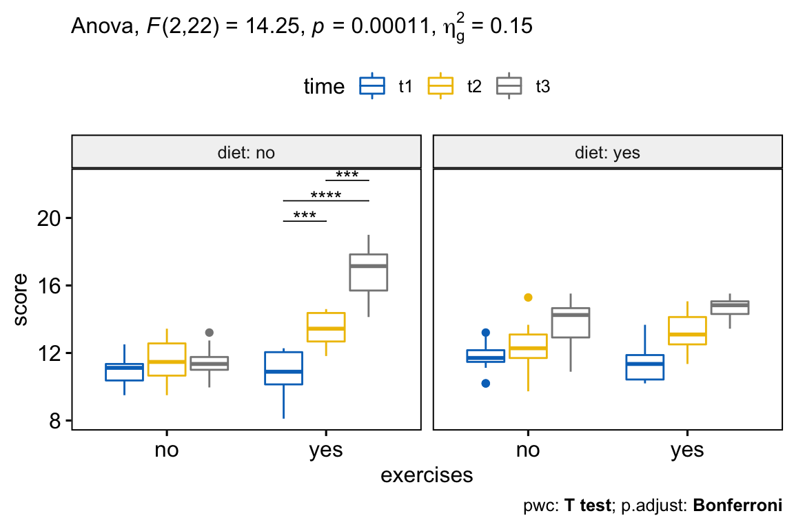
Create box plots:
bxp <- ggboxplot(
  weightloss, x = "exercises", y = "score",
  color = "time", palette = "jco",
  facet.by = "diet", short.panel.labs = FALSE
  )
bxp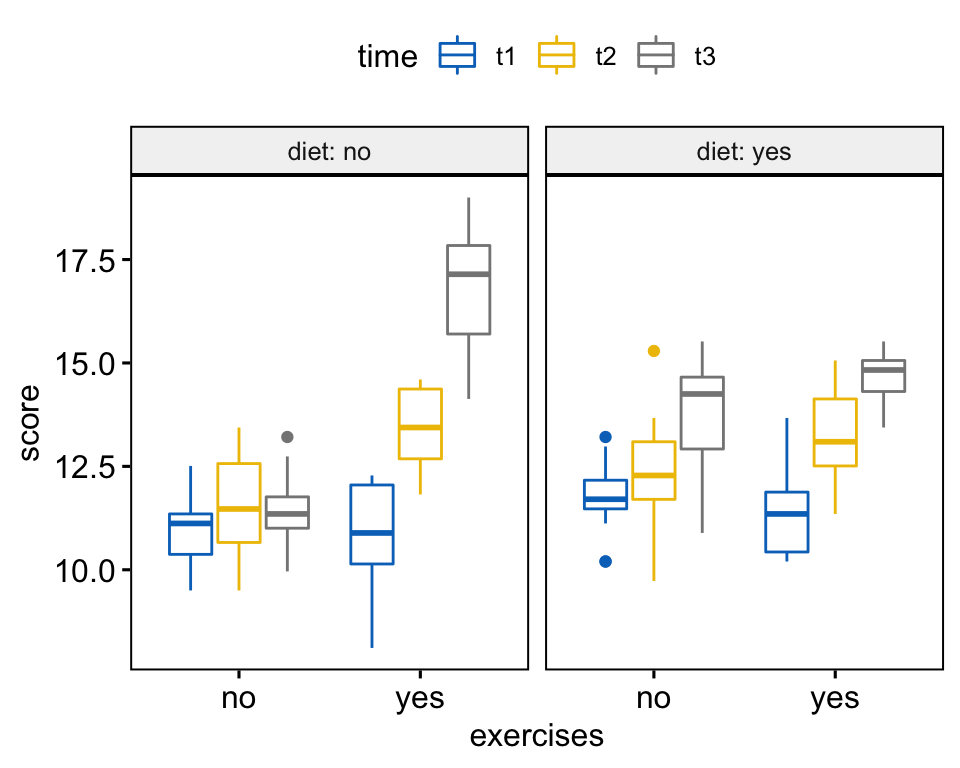
Check assumptions
Outliers
weightloss %>%
  group_by(diet, exercises, time) %>%
  identify_outliers(score)
## # A tibble: 5 x 7
## diet exercises time id score is.outlier is.extreme
## <fct> <fct> <fct> <fct> <dbl> <lgl> <lgl>
## 1 no no t3 2 13.2 TRUE FALSE
## 2 yes no t1 1 10.2 TRUE FALSE
## 3 yes no t1 3 13.2 TRUE FALSE
## 4 yes no t1 4 10.2 TRUE FALSE
## 5 yes no t2 10 15.3 TRUE FALSEThere were no extreme outliers.
Normality assumption
Compute Shapiro-Wilk test for each combinations of factor levels:
weightloss %>%
  group_by(diet, exercises, time) %>%
  shapiro_test(score)
## # A tibble: 12 x 6
## diet exercises time variable statistic p
## <fct> <fct> <fct> <chr> <dbl> <dbl>
## 1 no no t1 score 0.917 0.264
## 2 no no t2 score 0.957 0.743
## 3 no no t3 score 0.965 0.851
## 4 no yes t1 score 0.922 0.306
## 5 no yes t2 score 0.912 0.229
## 6 no yes t3 score 0.953 0.674
## # … with 6 more rowsThe weight loss score was normally distributed, as assessed by Shapiro-Wilk’s test of normality (p > .05).
Create QQ plot for each cell of design:
ggqqplot(weightloss, "score", ggtheme = theme_bw()) +
  facet_grid(diet + exercises ~ time, labeller = "label_both")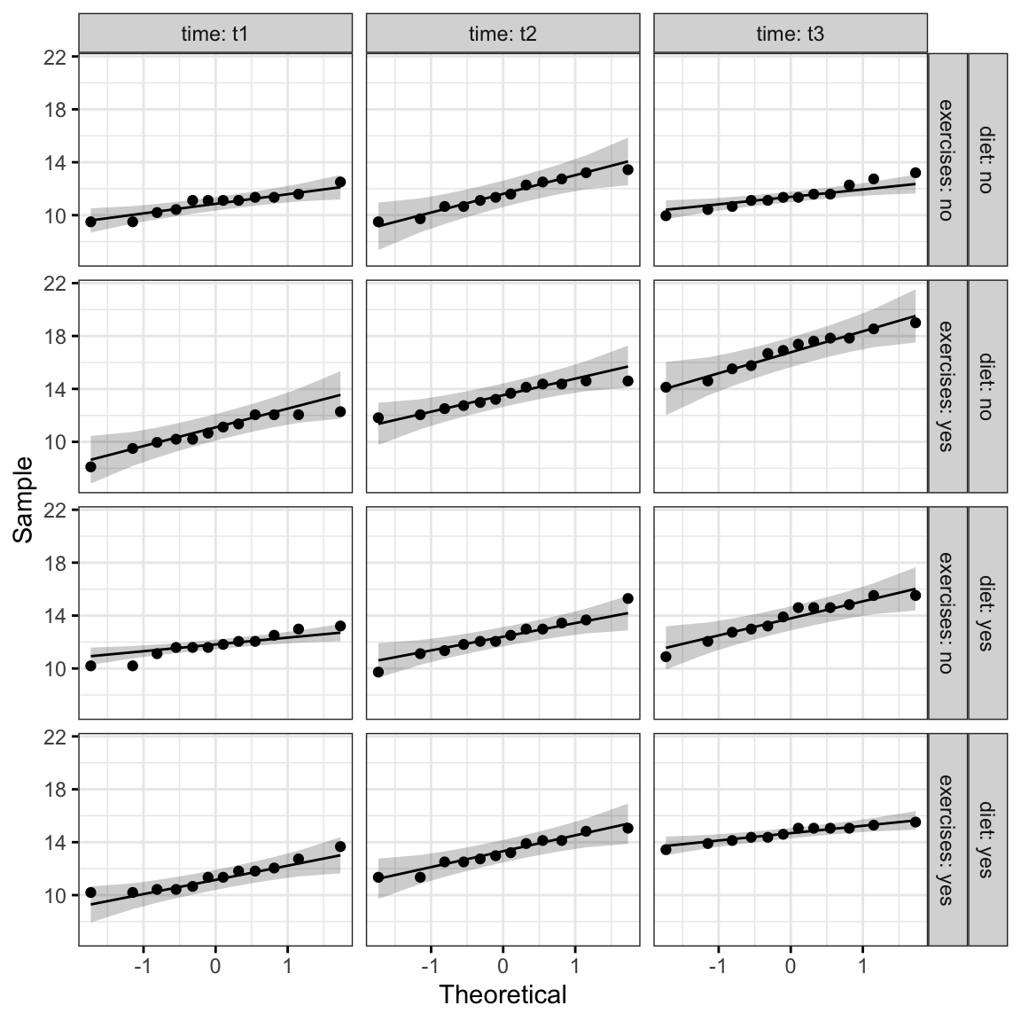
From the plot above, as all the points fall approximately along the reference line, we can assume normality.
Computation
res.aov <- anova_test(
  data = weightloss, dv = score, wid = id,
  within = c(diet, exercises, time)
  )
get_anova_table(res.aov)
## ANOVA Table (type III tests)
##
## Effect DFn DFd F p p<.05 ges
## 1 diet 1.00 11.0 6.021 3.20e-02 * 0.028
## 2 exercises 1.00 11.0 58.928 9.65e-06 * 0.284
## 3 time 2.00 22.0 110.942 3.22e-12 * 0.541
## 4 diet:exercises 1.00 11.0 75.356 2.98e-06 * 0.157
## 5 diet:time 1.38 15.2 0.603 5.01e-01 0.013
## 6 exercises:time 2.00 22.0 20.826 8.41e-06 * 0.274
## 7 diet:exercises:time 2.00 22.0 14.246 1.07e-04 * 0.147From the output above, it can be seen that there is a statistically significant three-way interactions between diet, exercises and time, F(2, 22) = 14.24, p = 0.00011.
Note that, if the three-way interaction is not statistically significant, you need to consult the two-way interactions in the output.
In our example, there was a statistically significant two-way diet:exercises interaction (p < 0.0001), and two-way exercises:time (p < 0.0001). The two-way diet:time interaction was not statistically significant (p = 0.5).
Post-hoc tests
If there is a significant three-way interaction effect, you can decompose it into:
- Simple two-way interaction: run two-way interaction at each level of third variable,
- Simple simple main effect: run one-way model at each level of second variable, and
- simple simple pairwise comparisons: run pairwise or other post-hoc comparisons if necessary.
Compute simple two-way interaction
You are free to decide which two variables will form the simple two-way interactions and which variable will act as the third (moderator) variable. In the following R code, we have considered the simple two-way interaction of exercises*time at each level of diet.
Group the data by diet and analyze the simple two-way interaction between exercises and time:
# Two-way ANOVA at each diet level
two.way <- weightloss %>%
  group_by(diet) %>%
  anova_test(dv = score, wid = id, within = c(exercises, time))
two.way
## # A tibble: 2 x 2
## diet anova
## <fct> <list>
## 1 no <anov_tst>
## 2 yes <anov_tst># Extract anova table
get_anova_table(two.way)## # A tibble: 6 x 8
## diet Effect DFn DFd F p `p<.05` ges
## <fct> <chr> <dbl> <dbl> <dbl> <dbl> <chr> <dbl>
## 1 no exercises 1 11 72.8 3.53e- 6 * 0.526
## 2 no time 2 22 71.7 2.32e-10 * 0.587
## 3 no exercises:time 2 22 28.9 6.92e- 7 * 0.504
## 4 yes exercises 1 11 13.4 4.00e- 3 * 0.038
## 5 yes time 2 22 20.5 9.30e- 6 * 0.49
## 6 yes exercises:time 2 22 2.57 9.90e- 2 "" 0.06There was a statistically significant simple two-way interaction between exercises and time for “diet no” trial, F(2, 22) = 28.9, p < 0.0001, but not for “diet yes” trial, F(2, 22) = 2.6, p = 0.099.
Note that, it’s recommended to adjust the p-value for multiple testing. One common approach is to apply a Bonferroni adjustment to downgrade the level at which you declare statistical significance.
This can be done by dividing the current level you declare statistical significance at (i.e., p < 0.05) by the number of simple two-way interaction you are computing (i.e., 2).
Thus, you only declare a two-way interaction as statistically significant when p < 0.025 (i.e., p < 0.05/2). Applying this to our current example, we would still make the same conclusions.
Compute simple simple main effect
A statistically significant simple two-way interaction can be followed up with simple simple main effects.
In our example, you could therefore investigate the effect of time on the weight loss score at every level of exercises or investigate the effect of exercises at every level of time.
You will only need to consider the result of the simple simple main effect analyses for the “diet no” trial as this was the only simple two-way interaction that was statistically significant (see previous section).
Group the data by diet and exercises, and analyze the simple main effect of time. The Bonferroni adjustment will be considered leading to statistical significance being accepted at the p < 0.025 level (that is 0.05 divided by the number of tests (here 2) considered for “diet:no” trial.
# Effect of time at each diet X exercises cells
time.effect <- weightloss %>%
  group_by(diet, exercises) %>%
  anova_test(dv = score, wid = id, within = time)
time.effect
## # A tibble: 4 x 3
## diet exercises anova
## <fct> <fct> <list>
## 1 no no <anov_tst>
## 2 no yes <anov_tst>
## 3 yes no <anov_tst>
## 4 yes yes <anov_tst># Extract anova table
get_anova_table(time.effect) %>%
filter(diet == "no")## # A tibble: 2 x 9
## diet exercises Effect DFn DFd F p `p<.05` ges
## <fct> <fct> <chr> <dbl> <dbl> <dbl> <dbl> <chr> <dbl>
## 1 no no time 2 22 1.32 2.86e- 1 "" 0.075
## 2 no yes time 2 22 78.8 9.30e-11 * 0.801There was a statistically significant simple simple main effect of time on weight loss score for “diet:no,exercises:yes” group (p < 0.0001), but not for when neither diet nor exercises was performed (p = 0.286).
Compute simple simple comparisons
A statistically significant simple simple main effect can be followed up by multiple pairwise comparisons to determine which group means are different.
Group the data by diet and exercises, and perform pairwise comparisons between time points with Bonferroni adjustment:
# Pairwise comparisons
pwc <- weightloss %>%
  group_by(diet, exercises) %>%
  pairwise_t_test(score ~ time, paired = TRUE, p.adjust.method = "bonferroni") %>%
  select(-df, -statistic) # Remove details
# Show comparison results for "diet:no,exercises:yes" groups
pwc %>% filter(diet == "no", exercises == "yes") %>%
  select(-p)     # remove p columns
## # A tibble: 3 x 9
## diet exercises .y. group1 group2 n1 n2 p.adj p.adj.signif
## <fct> <fct> <chr> <chr> <chr> <int> <int> <dbl> <chr>
## 1 no yes score t1 t2 12 12 0.000741 ***
## 2 no yes score t1 t3 12 12 0.0000000121 ****
## 3 no yes score t2 t3 12 12 0.000257 ***In the pairwise comparisons table above, we are interested only in the simple simple comparisons for “diet:no,exercises:yes” groups. In our example, there are three possible combinations of group differences. We could report the pairwise comparison results as follow.
All simple simple pairwise comparisons were run between the different time points for “diet:no,exercises:yes” trial. The Bonferroni adjustment was applied. The mean weight loss score was significantly different in all time point comparisons when exercises are performed (p < 0.05).
Report
A three-way repeated measures ANOVA was performed to evaluate the effects of diet, exercises and time on weight loss. There was a statistically significant three-way interaction between diet, exercises and time, F(2, 22) = 14.2, p = 0.00011.
For the simple two-way interactions and simple simple main effects analyses, a Bonferroni adjustment was applied leading to statistical significance being accepted at the p < 0.025 level.
There was a statistically significant simple two-way interaction between exercises and time for “diet no” trial, F(2, 22) = 28.9, p < 0.0001, but not for “diet yes”" trial, F(2, 22) = 2.6, p = 0.099.
There was a statistically significant simple simple main effect of time on weight loss score for “diet:no,exercises:yes” trial (p < 0.0001), but not for when neither diet nor exercises was performed (p = 0.286).
All simple simple pairwise comparisons were run between the different time points for “diet:no,exercises:yes” trial with a Bonferroni adjustment applied. The mean weight loss score was significantly different in all time point comparisons when exercises are performed (p < 0.05).
# Visualization: box plots with p-values
pwc <- pwc %>% add_xy_position(x = "exercises")
pwc.filtered <- pwc %>%
  filter(diet == "no", exercises == "yes")
bxp +
  stat_pvalue_manual(pwc.filtered, tip.length = 0, hide.ns = TRUE) +
  labs(
    subtitle = get_test_label(res.aov, detailed = TRUE),
    caption = get_pwc_label(pwc)
  )
Summary
This chapter describes how to compute, interpret and report repeated measures ANOVA in R. We also explain the assumptions made by repeated measures ANOVA tests and provide practical examples of R codes to check whether the test assumptions are met.
Recommended for you
This section contains best data science and self-development resources to help you on your path.
Books - Data Science
Our Books
- Practical Guide to Cluster Analysis in R by A. Kassambara (Datanovia)
- Practical Guide To Principal Component Methods in R by A. Kassambara (Datanovia)
- Machine Learning Essentials: Practical Guide in R by A. Kassambara (Datanovia)
- R Graphics Essentials for Great Data Visualization by A. Kassambara (Datanovia)
- GGPlot2 Essentials for Great Data Visualization in R by A. Kassambara (Datanovia)
- Network Analysis and Visualization in R by A. Kassambara (Datanovia)
- Practical Statistics in R for Comparing Groups: Numerical Variables by A. Kassambara (Datanovia)
- Inter-Rater Reliability Essentials: Practical Guide in R by A. Kassambara (Datanovia)
Others
- R for Data Science: Import, Tidy, Transform, Visualize, and Model Data by Hadley Wickham & Garrett Grolemund
- Hands-On Machine Learning with Scikit-Learn, Keras, and TensorFlow: Concepts, Tools, and Techniques to Build Intelligent Systems by Aurelien Géron
- Practical Statistics for Data Scientists: 50 Essential Concepts by Peter Bruce & Andrew Bruce
- Hands-On Programming with R: Write Your Own Functions And Simulations by Garrett Grolemund & Hadley Wickham
- An Introduction to Statistical Learning: with Applications in R by Gareth James et al.
- Deep Learning with R by François Chollet & J.J. Allaire
- Deep Learning with Python by François Chollet
Version:
 Français

What an excellent resource! Thank you for providing this website to the public. I will recommend it to my students, too.
Thank you for your positive feedback, highly appreciated!
Thank you so much, helps a lot! One thing that might be relevant for some people is when to use between subjects instead of within subjects. But, the main thing is that this is the best source for doing these types of analyses I could find on the web, so great job!
Thank you for your positive feedback! I’ll take your suggestion into account in the next update
Hi! Thanks for such a wonderfully written intro to the topic with easy to read R code – a breath of fresh air!
I had a question about the following section:
“It’s also possible to keep the outliers in the data and perform robust ANOVA test using the WRS2 package.”
I’ve been reading the Mair et al (2018) paper that introduces WRS2 titled “Robust Statistical Methods Using WRS2” and specifically section 6.1 on Repeated Measurement and Mixed ANOVA Designs that introduces the function I believe you are referring to (rmanova). However, the authors state that the function provides a “robust heteroscedastic repeated measurement ANOVA based on the trimmed means” which defaults to 20%. Would this trimmed mean not remove the outliers, rather than keep them?
I’d be grateful for any help you could offer, maybe I’ve got the wrong function or the wrong end of the stick?
Cheers!
Error in lm.fit(x, y, offset = offset, singular.ok = singular.ok, …) :
0 (non-NA) cases
Hi, could you please provide a reproducible example?
I am also having this problem, though the dataset you use in the example works fine :(.
Data:
id treatment t1 t2 t3
1 Diet 3 7 7
2 Diet 5 7 7
3 Diet 2 7 8
4 Diet 4 3 4
5 Diet 5 4 4
6 Diet 3 4 4
7 Diet 5 9 9
8 Diet 3 4 4
9 Diet 3 8 8
10 Diet 5 4 4
147 ctr 5 3 3
148 ctr 4 6 6
149 ctr 7 8 8
150 ctr 3 2 2
151 ctr 7 4 4
152 ctr 3 6 6
153 ctr 5 5 5
154 ctr 4 7 7
155 ctr 5 1 1
157 ctr 6 5 5
zna <- read.csv("zero_na.csv")
zna % gather(key = “time”, value = “score”, t1, t2, t3) %>%
convert_as_factor(id, time)
res.aov <- anova_test(
data = zna, dv = score, wid = id,
within = c(treatment, time)
)
get_anova_table(res.aov)
I got this error message when I tried to do two-way anova. My case was different from the example because I had different participants in all (three) groups; I think this is why I got an error.
Eventually, I analysed my data using lme function and setting a unique random effect to each participant.
If you have repeated measures on three different groups of participant, then it looks like you have a mixed two-way ANOVA design. https://www.datanovia.com/en/lessons/mixed-anova-in-r/
I got the same error again and again. I was following all the steps. Later I discovered. that my data frame consisted of 2 additional variables that were not used. For some strange reasons, if I deleted the unwanted variables, the error no longer came. It is difficult to explain this situation.
This issue has been fixed in the latest dev version of the rstatix package: https://github.com/kassambara/rstatix/issues/55
Hi
Can you please guide me on how to arrange data for three-way repeated measure Anova when you have 5 genotypes, three treatments and 7 measured parameters on 6 times (after 10 days) during crop life span.
Hello! Thank’s a lot for this article, it helps a lot. I’m using three-way anova for my dataset and when I run function ‘anova_test’ (opy from this text here) i get an error: ‘Each row of output must be identified by a unique combination of keys.
Keys are shared for 715 rows:’. Maybe you could help and tell me what’s going on?
My function looks like:
aov <- anova_test(data=rtdata, dv=rt, wid=part, within=c(mod_sm, con, resp))
where:
rtdata – data in long format
part – factor, participant code from 1 to 12; each participant got 60 trials, so his code repeats 60 times in dataset
mod_sm – text, levels 'pos' and 'neg'
con – text, 'n' and 'y'
resp – factor, 1 and 2
Thank you!
Hey May, did you manage to figure out how to fix this issue? I have exactly the same issue and my data structure is similar.
I have been trying to do a two-way repeated samples and spent many hours until I worked out what was wrong – my control and treatment groups aren’t the same, so don’t have the same ids repeated. So it is not “ctr” followed by “Diet” for the same subjects but separate subject
Can you comment on how this would work? What kind of test would it be? Thanks!
If you have repeated measures on different groups of participants, then it corresponds to a mixed measures ANOVA design. This article might help: https://www.datanovia.com/en/lessons/mixed-anova-in-r/
Very informative!
I’ll recommend this guide everywhere
Thank you for your positive feedback, highly appreciated!
Hi, I’ve been trying for days to run the 3-way repeated measures ANOVA for my dataset in a long format with 2x treatment groups (temp & region) and then a time group (T0, T1, T2, T3). Whenever I run the ANOVA, I get the same error message that has been mentioned above and in many other R forums (StackExchange, etc.), although I’ve not as yet seen a solution as my data does not contain any null data and all my groups are in factor format (I’ve also tried them in numeric format without luck):
Error in lm.fit(x, y, offset = offset, singular.ok = singular.ok, …) :
0 (non-NA) cases
Can you help or offer any suggestions that I might not have tried?
It seems that you have a mixed design, so try a mixed anova test as described at: https://www.datanovia.com/en/lessons/mixed-anova-in-r/.
Please provide a reproducible example with a demo dataset so that I can help. Please consider this article for inserting a reproducible R script in datanovia comments : https://www.datanovia.com/en/blog/publish-reproducible-examples-from-r-to-datanovia-website/
Hi Kassambara,
Thank you for your work.
It seems there are a conflict with the packtage “tidyverse” and “rstatix”.
This conflict may explain the errors :
– “Error in lm.fit(x, y, offset = offset, singular.ok = singular.ok, …) :
0 (non-NA) cases”
– “Error: Unknown column `ID`”
To remedy this i use the package “conflict_prefer”.
Moreover, the first error also appears when i have unused columns (Factor or Numeric) in my dataframe. When i remove unused columns, the anova_test work fine.
Hi, thank you for your input. I can’t reproduce this error.
Would you please provide a reproducible R script so that I can fix this issue.
Thanks, the root cause is fixed now in the latest dev version of the
rstatix, which can be installed using:devtools::install_github("kassambara/rstatix").The issue is documented at: rstatix fails to compute repeated measures when unused columns are present in the input
Hi great article!
Tried to produce graph report of one-way anova and error at bottom of code came up.
PS_tried to install pubr but got nothing.
Thx JW
# Repeated One-Way ANOVA
res.aov <- anova_test(data = V3, dv=Data, wid=Name, within = Rep)
get_anova_table(res.aov)
# pairwise comparisons
pwc %
pairwise_t_test(
Data ~ Rep, paired = TRUE,
p.adjust.method = “bonferroni”
)
pwc
# Visualization: box plots with p-values
pwc % add_xy_position(x = “Rep”)
bxp +
stat_pvalue_manual(pwc) +
labs(
subtitle = get_test_label(res.aov, detailed = TRUE),
caption = get_pwc_label(pwc)
Error in bxp + stat_pvalue_manual(pwc) + labs(subtitle = get_test_label(res.aov, :
non-numeric argument to binary operator
Hi,
It should be possible to install pubr using `devtools::install_github(“kassambara/pubr”)`.
In order efficiently I need a reproducible example with a demo data.
Thanks
Really great examples that are well explained.
My issue is when trying to visualize the final box plot with the p-values for any of the examples. I receive the following error each time:
Error in f(…) :
Can only handle data with groups that are plotted on the x-axis
In addition: Warning messages:
1: Ignoring unknown parameters: hide.ns
2: Ignoring unknown aesthetics: xmin, xmax, annotations, y_position
Please advise and what the issue may be. Thank you
Please make sure you have the latest version of the rstatix and the ggpubr packages
Thanks for the excellent tutorial! I got the same error with data visualization. Have you figured out the potential issue with this error?
Hi Kassambara,
Thanks a lot for your input, it’s really helpful. I have one question that the output of two-way repeated ANOVA analysis in R is not consistent with the results obtained in SPSS, what kind of reason do you think can explain this difference? thanks in advance.
Hi!
After checking, I found that the output of SPSS and rstatix are the same when considering the rstatix raw output (
res.aov).When displaying the ANOVA table using the function
get_anova_table(res.aov), the sphericity correction is automatically applied when the sphericity can’t be assumed.The sphericity assumption can be checked using the Mauchly’s test of sphericity, which is automatically reported when using the R function
rstatix::anova_test()Hey, great tutorial! This is by far the easiest and most understandable approach I have found.
I am working on my bachelor thesis and using R instead of SPSS. I need to calculate several 2 way repeated Anovas and rstatix seems more than handy atm. However, I cannot find any explanation of the output: What is the value of DFd? I calculated a oneway repeated Anova with 1 factor of 3 levels. DFn seems to be the degree of freedom between the levels (2) and DFd’s value is 30.
I have 16 participants and I dont know how the degrees of freedom could go up this far… Though, my statistics courses were 2 years ago…
Thanks in advance!
Hi, thank you for the positive feedback!
DFnis the Degrees of Freedom in the numerator (i.e. DF for the effect of the experiment);DFdDegrees of Freedom in the denominator (i.e., DF for the residual, DFd Degrees of Freedom in the denominator (i.e., DF error)). This is explained in the documentation of anova_summary(), but obviously, we should clarify it in the current blog post.If only one factor is repeated measures, the number of degrees of freedom (DFd) can be calculated as
(n-1)(a-1), wherenis the number of participants andais the number of levels of the repeated measures factor.If two factors are repeated measures, the number of degrees of freedom (DFd) for the two-way interaction term can be calculated as
(n-1)(a-1)(b-1)wherenis the number of participants,ais the number of levels one factor, andbis the number of levels of the other factor. Note that, a sphericity correction is applied, when the sphericity assumtion is not met, resulting in a fractional degres of freedom.Thank you so much for the fast response!
(16-1) (3-2) = 30 should be fine then.
Due to the pandemic I was not able to test all participants and I am allowed to set the alpha level to 0.10 instead of 0.05. Is it possible to adjust it within your package, so that get_anova_table() marks p<.10 with * ?
Even if not, your package worked great so far. Thanks again!
It’s possible to do something like this:
Hi,
Thank you very much for your website! It helps a lot with my analysis works.
I have one question, after running the rstatix::anova_test() code, it only shows the ANOVA table. I would like to check the sphericity assumption for my data but could not find it in the anova_test result. (I have tried to use your example data (selfesteem2) to do the analysis and can check the sphericity assumption in the ANOVA table. So I think the problem is from my data.) Do you have any idea what would be the possible reasons? (I run the two-wat rmANOVA) Thank you very much again!!
Note that the the Mauchly’s Test of Sphericity is only reported for variables or effects with >2 levels because sphericity necessarily holds for effects with only 2 levels Read more: Mauchly’s Test of Sphericity in R. Does your within-measures variable contains only two levels?
Hi, thank you very much for your response! I found the solution from your answer in the previous question asked by Jack. My data is a mixed two-way ANOVA design (have 3 treatments). After changing the analysis method I get the Mauchly’s Test of Sphericity in my result. Thank you very much for your help!
There are non-parametric method for 2/3 way repeated ANOVA. It’s WTS (Wald-Type Statistics), permuted WTS, ATS (ANOVA-Type Statistics) and ART (Aligned-Rank Transform) ANOVA. Both methods are available in R, not to mention Conover’s ANOVA (on “classic” ranks). Please check: nparLD, GFD, rankFD, ARTool and MANOVA packages.
Thank you for your input, very useful and instructive. Obviously, we’ll write on these packages!
Hi! Thanks for this beautiful and useful explanation.
I have a question regarding treating outliers:
You say that if outliers are NOT extreme you keep in the analysis right?
If I want to remove outliers from my dataset and compute anova, which is the command to remove them?
Thank you in advance.
Sara
Thank you Sara, for your positive feedback, highly appreciated!
Once you identified outliers, you can filter out the corresponding samples (before computing ANOVA), by using the R function dplyr::filter().
Excellent guide and your hard work is very much appreciated.
I am getting the same error code as several others:
Error in lm.fit(x, y, offset = offset, singular.ok = singular.ok, …) :
0 (non-NA) cases
I have tried using the Mixed ANOVA, but that will not run either. I also tried using the “conflict_prefer”as a poster suggested, but that does not help either. There are no NA’s in any of my data columns. I have three categorical IVs (speaker, complexity, format) and not sure where I am going wrong.
I will try and post a reproducible R script here later.
Thanks for the help and thanks for the excellent guides.
I appreciate positive feedback.
If you can send to me a reproducible script with your data, I will be able to check closely this issue.
Thanks
Please consider providing reproducible example with a demo data as described at : https://www.datanovia.com/en/blog/publish-reproducible-examples-from-r-to-datanovia-website/
Thanks, fixed now in the latest dev version of the
rstatix, which can be installed using:devtools::install_github("kassambara/rstatix").The issue is documented at: rstatix fails to compute repeated measures when unused columns are present in the input
Great article! Only one aspect, a non-significant p-value for the Shapiro test doesn’t guarantee that the data is normally distributed. It may happen that the data you have is not enough to reject the null. The q-q plot is always a good double check as you did!
Thank you for your input!
Hi,
Thank for build so amazing tool!
My question is: My data is not perfectly normal and I have some outliers, but results are consistent. In these cases, I am more calm if I can see model residuals. Any way to obtain anova_test residuals?
The returned object by the
anova_test()function has an attribute called args, which is a list holding the arguments used to fit the ANOVA model, including: data, dv, within, between, type, model, etc.You can access to the residuals as follow:
residuals(attr(res.aov, "args")$model)Are you the best? maybe… jejeje
Thanks!
Hi, I’m trying to run Two-way repeated measures ANOVA but I kept getting this message:
Error in lm.fit(x, y, offset = offset, singular.ok = singular.ok, …) :
0 (non-NA) cases
And I don’t see any missing data for my data. This is what I did:
res.aov <- anova_test(
data = Tab14_4, dv = Behavior, wid = Subject,
within = c(Group, Interval)
)
Pls help!
Please send a demo data so that I can reproduce the error and help.
Thanks
Is this related to the issue is documented at: rstatix fails to compute repeated measures when unused columns are present in the input
If yes, then it is fixed now in the latest dev version of the
rstatix, which can be installed using:devtools::install_github("kassambara/rstatix").Hi, I’m also trying to run Two-way repeated measures ANOVA like Danny but I kept getting this message:
Error in lm.fit(x, y, offset = offset, singular.ok = singular.ok, …) :
0 (non-NA) cases
And I don’t see any missing data for my data. This is what I did:
anova_test(data = mydata2,dv = Score,wid = Subjects,within = c(Drinks,Gender))
May I sent my demo to you?
I really need your help!
Hi, In order to fix this issue I need a reproducible example with a data. Would you like to send your data with a reproducible R script?
Hi there, I am also experiencing the same issue as Peggy and Danny. I have spent hours trying to get this to work (after it had successfully worked many times the other day) and have had no luck. It works perfectly fine with the data presented on this site, but is no longer working with my data. I also have no missing cases present within my dataset.
res.aov <- anova_test(data = newanova, dv = score, wid = id, within = c(treatment, time))
Error in lm.fit(x, y, offset = offset, singular.ok = singular.ok, …) :
0 (non-NA) cases
Please help!
Hi, In order to fix this issue I need a reproducible example with a data. Would you like to send your data with a reproducible R script?
Have you find a solution? I am in the same situation.
If the data is an imbalance between groups, Does this still work?
Cause in my data, the first group has 100 samples, the second group only has 10 samples
I am looking forward to your reply! Thank you very much!
Hi ! Thank you so much for this explanation. I found this so helpful.
However, I have some issues when doing this with my data. I removed the NA from my dataset. I tried to do as your “example 1: Reproducible R script using R built-in data” but I am not sure this works… I had error mesage while running “pubr::render_r()”.
My independent variable is secondhand smoke (SHS yes or no) and cognitive test score at 2 points of time.
When I compute the anova test. I got this message:
“Error in lm.fit(x, y, offset = offset, singular.ok = singular.ok, …) : 0 (non-NA) cases”
# Computation
res.aov2 <- anova_test(data = ds, dv = score, wid = ID,
within = c(SHSCAT, time))
get_anova_table(res.aov2)
Then when I want to see the effect of independent variable at each time point, I got an error message:
"Error: Problem with `mutate()` input `data`. x 0 (non-NA) cases i Input `data` is `map(.data$data, .f, …)`"
# Effect of SHS smoke at each time point
one.way % group_by(time) %>%
anova_test(dv = score, wid = ID, within = SHSCAT) %>%
get_anova_table() %>%
adjust_pvalue(method = “bonferroni”)
I really need your help. I tried to find other codes, to watch videos, but nothing fixed my problem.
Thank you for time.
Please, provide your data and the R script you used so that we can help, thanks
Hello,
thank you for the great article! I would like to use this procedure in my master’s thesis. Do you have some references to literature for me ?
Thank you so much!
I need references for the pairwise paired t-tests and the one way ANOVA with repeated measures. Thank you so much!
Hi there, is there any way to hide ” eta square” value when adding pvalues on ggplot?
adding Cohen.d instead of eta square ?
Hey Kassambara,
Thanks for your amazing instructions on repeated measures ANOVA. However, like many others it seem, I also receive the error message:
“Error in lm.fit(x, y, offset = offset, singular.ok = singular.ok, …) :
0 (non-NA) cases”
when trying to run the 2-way repeated ANOVA. I have removed any unused variables from the data set and tried running the: “suppressPackageStartupMessages(library(rstatix))” as well. And if I try to install your rstatix package, I get this message ‘kassambara/rstatix’ is not available (for R version 4.0.1) . I have just updated my Rstudio and believe I have the newest version?
My data looks like this:
>head(data)
ID Site Day Sediment
1 1 Site 1 Day 1 5.5
2 2 Site 1 Day 1 -2.75
3 3 Site 1 Day 1 -9.65
4 1 Site 1 Day 3 9.3
5 2 Site 1 Day 3 -0.2
6 3 Site 1 Day 3 -2.45
I have three Sites (site 1, Site 2, Site 3) which are measured 5 times (Day 1, Day 3, Day 7, Day 14, Day 33) and my dependent variable is sediment levels (Sediment).
I would be very grateful if you can help me solve this problem.
Kind regards
Thank you for the feedback! This has been fixed now in the latest dev version (see https://github.com/kassambara/rstatix/issues/55), which can be installed using devtools::install_github(“kassambara/rstatix”)
Hi Kassambara, thank you for your great explanations and examples! I would have one question on you. How to compare more than two treatment groups in 2-way repeated-measures ANOVA?
I am trying to do a two-way repeated-measures ANOVA, only I have 3 treatment groups (independent variable 1) over time (independent variable 2). I got significant two-way interaction and a simple main effect. You used paired t-test in your example to compare the treatment groups so I tried anova_test instead. That was significant for some of the time points. But now, I cannot figure out how to do a posthoc Tuckey to know how they differ? I can’t get TukeyHSD working with the output from anova_test (I always used aov function, but there you cannot use group_by()).
I ran my anova as follows:
comparison %
group_by(time) %>%
anova_test(dependent variable ~ treatment) %>%
get_anova_table() %>%
adjust_pvalue(method = “bonferroni”)
Kind regards
Hi Kassambara,
Thanks for the amazing tutorial!
I have a question that whether partial counterbalance design can be analyzed with anova_test().
I have two IV: tool (N, R, S) and topic (T, F, K), each one has three levels. If it is a complete counterbalancing design, each participants should has 9 treatment. But that is impratical. So in my study, each participant experienced 3 treatment (e.g. [NT, RF, SK], [RT, NK, SF]), each tool and topic only appear once for each participant.
When I used anova_test(), I got the same error as above: Error in lm.fit(x, y, offset = offset, singular.ok = singular.ok, …) : 0 (non-NA) cases. I do not have NA in my dataset.
Should I use mixed model instead? But every IV is within subject variable, I think I should use repeated measurement ANOVA.
If it does not make sense I will provide reproducible demo data.
Hi, this issue seems to be related to the issue described at https://github.com/kassambara/rstatix/issues/55, which has been fixed in the rstatix dev version available on Github. Please make sure you have installed the latest dev version of the rstatix package.
Hi Kassambara,
I installed the package using devtools::install_github(“kassambara/rstatix”)
But still get this error.
Here is a script:
demo <- data.frame(id = c(1L,1L,1L,2L,2L,
2L,3L,3L,3L,4L,4L,4L,5L,5L,5L,6L,6L,6L,
7L,7L,7L,8L,8L,8L,9L,9L,9L,10L,10L,10L,
11L,11L,11L,12L,12L,12L,13L,13L,13L,14L,14L,
14L,15L,15L,15L,16L,16L,16L,17L,17L,17L,
18L,18L,18L,19L,19L,19L,20L,20L,20L,21L,21L,
21L,22L,22L,22L,23L,23L,23L,24L,24L,24L,
25L,25L,25L,26L,26L,26L,27L,27L,27L,28L,
28L,28L,29L,29L,29L,30L,30L,30L,31L,31L,31L,
32L,32L,32L,33L,33L,33L,34L,34L,34L,35L,
35L,35L,36L,36L,36L),
result = c(4,4,4,4,4.5,3.5,
4,2,4,4,2,4,4,4,4,2,3.5,3,6,1,4,4,
4.5,3.5,3.5,2,5.5,5.5,6,6.5,3,2,5,1,6,
6.5,3.5,4.5,4.5,3,5,5.5,2,2,3.5,2,5,5,4,
6,7,5,5,5,3,5,5,4,4.5,5,4.5,6.5,6.5,5,
4.5,3,5,5,6,6,6,7,4,5.5,5,6,6,5.5,2,
4.5,5,1,7,7,1,4,4.5,3,5,6,6,2.5,7,3,3,
5,2,5,7,1.5,2,2,1.5,4.5,5,1,3,1),
topic = c(1L,2L,3L,2L,3L,
1L,3L,1L,2L,3L,2L,1L,2L,1L,3L,1L,3L,2L,
2L,3L,1L,3L,1L,2L,1L,2L,3L,1L,3L,2L,3L,
2L,1L,2L,1L,3L,3L,1L,2L,1L,2L,3L,2L,3L,
1L,2L,1L,3L,1L,3L,2L,3L,2L,1L,1L,2L,3L,
2L,3L,1L,3L,1L,2L,3L,2L,1L,2L,1L,3L,1L,
3L,2L,2L,3L,1L,3L,1L,2L,1L,2L,3L,1L,3L,
2L,3L,2L,1L,2L,1L,3L,3L,1L,2L,1L,2L,3L,
2L,3L,1L,2L,1L,3L,1L,3L,2L,3L,2L,1L),
tool = c(1L,2L,3L,2L,3L,
1L,3L,1L,2L,3L,2L,1L,2L,1L,3L,1L,3L,2L,
1L,2L,3L,2L,3L,1L,3L,1L,2L,3L,2L,1L,2L,
1L,3L,1L,3L,2L,1L,2L,3L,2L,3L,1L,3L,1L,
2L,3L,2L,1L,2L,1L,3L,1L,3L,2L,1L,2L,3L,
2L,3L,1L,3L,1L,2L,3L,2L,1L,2L,1L,3L,1L,
3L,2L,1L,2L,3L,2L,3L,1L,3L,1L,2L,3L,2L,
1L,2L,1L,3L,1L,3L,2L,1L,2L,3L,2L,3L,1L,
3L,1L,2L,3L,2L,1L,2L,1L,3L,1L,3L,2L),
trial = c(1L,2L,3L,1L,2L,
3L,1L,2L,3L,1L,2L,3L,1L,2L,3L,1L,2L,3L,
1L,2L,3L,1L,2L,3L,1L,2L,3L,1L,2L,3L,1L,
2L,3L,1L,2L,3L,1L,2L,3L,1L,2L,3L,1L,2L,
3L,1L,2L,3L,1L,2L,3L,1L,2L,3L,1L,2L,3L,
1L,2L,3L,1L,2L,3L,1L,2L,3L,1L,2L,3L,1L,
2L,3L,1L,2L,3L,1L,2L,3L,1L,2L,3L,1L,2L,
3L,1L,2L,3L,1L,2L,3L,1L,2L,3L,1L,2L,3L,
1L,2L,3L,1L,2L,3L,1L,2L,3L,1L,2L,3L)
)
anova_test(
data = demo, dv = result, wid = id,
within = c(topic, tool, trial)
)
Great tutorial and I’m getting some great plots. However, I have a small issue that I cannot resolve.
When doing a pairwise comparison and trying to add the significance to the boxplot using pairwise_t_test() and add_xy_position() the groups are ordered along the x axis alphabetically.
I have 3 groups: Normal, DblEl, ON. I want to display in that order but by default they are ordered DblEL, Normal, ON. I can alter the order in ggboxplot using order = c(‘Normal’, ‘DblEl’, ‘ON’), but cannot get the paired comparisons or their associated x numbering to match. Any ideas other than relabelling groups alphabetically? Thanks!
Hi,
I would suggest to prepare your data by defining the desired order of the factor variable levels before using any plotting or stat functions. For example, I would go as follow:
1/ Data preparation: defining the order of the variable
my_data$grouping_var = factor(my_data$grouping_var, levels = c(“Normal”, “DblEl”, “ON”))
2/ now you can use ggboxplot() or any stat functions. The defined factor levels at step 1 will be taken into account by all functions.
Thanks Alboukadel. Turns out r was automatically ascribing levels when I used read.csv(), seemingly alphabetically. I reassigned as you suggested and now works perfectly. Woop! Thanks.
Hi,
For one-way repeated measures ANOVA, is it possible to include the significance levels in the boxplot, but NOT when it is nonsignificant? In other words, is it possible to not to include it when it is “ns”.
Thanks,
Clara
Hi Kassambara,
I’m facing the same issue as many people here. I get the following error Error in lm.fit(x, y, offset = offset, singular.ok = singular.ok, …) :
0 (non-NA) cases
I don’t have any NAs in my dataset and I have downloaded the newest version you have suggested to other comments on here. Is there possibly a limit on data that can be managed? I have 5000+ data points. I want to compare two groups of stations within the same water body measured in 3 seasons and with a certain treatment. Hope you can help. Thanks.
Did you installed the dev version from Github? if yes and you still have the issue, please send to meby e-mail the data and the script you used so that I can help.
Hi,
I keep getting this error when I try to run two-way ANOVA: Error: Problem with `mutate()` input `data`.
x Can’t subset columns that don’t exist.
Can anyone help me with this??
I was getting the same error message, but I found it was due to group_by(). ungroup() stopped the error. I hope this will help.
Hi,
Thx a lot for the highly valuable info you’ve shared. I got a question mark that might also interest you for my own research purposes:
I’ve a dataset which has 2 tasks and each task comprises of 3 items. 40 participants complete these 6 items in total respectively. Their performance is assessed by 3 raters. My question is whether this task type have any impact on the participants performance. In this case, how should my SPSS data entry look like?
Thx a lot in advance!
Hi, thank you so much for this tutorial!
I have a question about Mauchly’s test. I am doing a two-way repeated measures ANOVA. Both the independent variables have more than two levels (5 and 6), but I cannot find any output for the sphericity assumptions. I’m running it like this:
res.aov <- anova_test(
data = G1_noid, dv = rating, wid = ppno,
within = c(instr_pair, pitch)
)
get_anova_table(res.aov)
Is there something I'm doing wrong here?
I also had a question for the normality assumption. As you can see there are a lot of levels, so the Shaprio Wilk is applied 30 times. Six of those came out significant. Does that mean I will have to run robust testing, even if relatively few groups were non-normal?
Thank you!
You just need to add a line after you have originally run the ANOVA with the name of your model (here res.aov). This will give you the Mauchly’s test result.
The pairwise t test results don’t match in R and SPSS. In SPSS, the pairwise comparison across time seems to be effected by the levels in the factor group’s levels which is not the case with R pairwise_t test function you mentioned. Any suggestion?
First of all, thank you very much Kassambara for this work! I am trying to run a repeated measure two-way ANOVA with my own data and I still seem to run into the error previously described by others;
Error in lm.fit(x, y, offset = offset, singular.ok = singular.ok, …) : )
0 (non-NA) cases
I have installed the latest dev version of the rstatix, however, that does not seem to solve the problem. Do you have any idea how to solve this issue? I would very much appreciate your help!
the code looks as followed:
my_data % sample_n_by(treatment, size = 1)
# Gather the columns t1, t2 and t3 into long format.
# Convert id and time into factor variables
my_data %
gather(key = “minute”, value = “score”, t1, t2) %>%
convert_as_factor(id, minute, treatment)
#Inspect some random rows of the data by groups
set.seed(123)
my_data %>% sample_n_by(treatment, minute, size = 1)
#summery of data
my_data %>%
group_by(treatment, minute) %>%
get_summary_stats(score, type = “mean_sd”)
#check for outlayers
my_data %>%
group_by(treatment, minute) %>%
identify_outliers(score)
#check for normality
my_data %>%
group_by(treatment, minute) %>%
shapiro_test(score)
#QQplot also check for normality
ggqqplot(my_data, “score”, ggtheme = theme_bw()) +
facet_grid(minute ~ treatment, labeller = “label_both”)
#if assumptions are met run repeated two way ANOVA
res.aov <- rstatix::anova_test(
data = my_data, dv = score, wid = id,
within = c(treatment, minute)
)
get_anova_table(res.aov)
data:
score id treatment minute
1 5.66666 1 ctrl t1
2 75.16670 3 ctrl t1
3 57.61120 5 ctrl t1
4 33.16670 7 ctrl t1
5 66.16660 9 ctrl t1
6 57.61110 11 ctrl t1
7 75.11110 13 ctrl t1
8 95.27780 15 ctrl t1
9 72.61110 17 ctrl t1
10 64.66670 19 ctrl t1
11 25.38890 21 ctrl t1
12 10.16670 23 ctrl t1
13 46.44440 4 Gs t1
14 3.05555 8 Gs t1
15 61.38880 12 Gs t1
16 74.61110 16 Gs t1
17 39.33340 18 Gs t1
18 81.55550 20 Gs t1
19 15.72220 22 Gs t1
20 49.72230 24 Gs t1
21 35.33330 25 Gs t1
22 37.72220 26 Gs t1
23 32.94440 1 ctrl t2
24 87.38890 3 ctrl t2
25 72.72230 5 ctrl t2
26 88.50000 7 ctrl t2
27 44.66660 9 ctrl t2
28 81.11120 11 ctrl t2
29 94.00000 13 ctrl t2
30 94.16650 15 ctrl t2
31 50.27760 17 ctrl t2
32 78.94450 19 ctrl t2
33 0.00000 21 ctrl t2
34 8.88888 23 ctrl t2
35 30.61110 4 Gs t2
36 0.00000 8 Gs t2
37 75.83330 12 Gs t2
38 69.77780 16 Gs t2
39 36.88890 18 Gs t2
40 3.05555 20 Gs t2
41 5.55555 22 Gs t2
42 29.88880 24 Gs t2
43 6.88888 25 Gs t2
44 23.27800 26 Gs t2
data.frame(
+ score = c(5.66666,75.1667,57.6112,33.1667,66.1666,
+ 57.6111,75.1111,95.2778,72.6111,64.6667,25.3889,10.1667,
+ 46.4444,3.05555,61.3888,74.6111,39.3334,81.5555,15.7222,
+ 49.7223,35.3333,37.7222,32.9444,87.3889,72.7223,88.5,
+ 44.6666,81.1112,94,94.1665,50.2776,78.9445,0,8.88888,
+ 30.6111,0,75.8333,69.7778,36.8889,3.05555,5.55555,29.8888,
+ 6.88888,23.278),
+ id = as.factor(c(“1″,”3″,”5″,”7″,”9”,
+ “11”,”13″,”15″,”17″,”19″,”21″,”23″,”4″,”8″,
+ “12”,”16″,”18″,”20″,”22″,”24″,”25″,”26″,”1″,
+ “3”,”5″,”7″,”9″,”11″,”13″,”15″,”17″,”19″,
+ “21”,”23″,”4″,”8″,”12″,”16″,”18″,”20″,”22″,
+ “24”,”25″,”26″)),
+ treatment = as.factor(c(“ctrl”,”ctrl”,”ctrl”,
+ “ctrl”,”ctrl”,”ctrl”,”ctrl”,”ctrl”,”ctrl”,
+ “ctrl”,”ctrl”,”ctrl”,”Gs”,”Gs”,”Gs”,”Gs”,”Gs”,
+ “Gs”,”Gs”,”Gs”,”Gs”,”Gs”,”ctrl”,”ctrl”,”ctrl”,
+ “ctrl”,”ctrl”,”ctrl”,”ctrl”,”ctrl”,”ctrl”,”ctrl”,
+ “ctrl”,”ctrl”,”Gs”,”Gs”,”Gs”,”Gs”,”Gs”,”Gs”,
+ “Gs”,”Gs”,”Gs”,”Gs”)),
+ minute = as.factor(c(“t1″,”t1″,”t1″,”t1”,
+ “t1″,”t1″,”t1″,”t1″,”t1″,”t1″,”t1″,”t1″,”t1”,
+ “t1″,”t1″,”t1″,”t1″,”t1″,”t1″,”t1″,”t1”,
+ “t1″,”t2″,”t2″,”t2″,”t2″,”t2″,”t2″,”t2″,”t2”,
+ “t2″,”t2″,”t2″,”t2″,”t2″,”t2″,”t2″,”t2″,”t2”,
+ “t2″,”t2″,”t2″,”t2″,”t2”))
+ )
First of all, thank you Kassambara for this work! I am trying to run a two way repeated measurement ANOVA with my own data but I still seem to run into error described above by others;
– Error in lm.fit(x, y, offset = offset, singular.ok = singular.ok, …) :
0 (non-NA) cases
I have updated the lasted dev version by running devtools::install_github(“kassambara/rstatix”). However, it still will give me the error. Do you have any idea how to fix this? I would very much appreciate your help!
Data:
data.frame(
+ score = c(5.66666,75.1667,57.6112,33.1667,66.1666,
+ 57.6111,75.1111,95.2778,72.6111,64.6667,25.3889,10.1667,
+ 46.4444,3.05555,61.3888,74.6111,39.3334,81.5555,15.7222,
+ 49.7223,35.3333,37.7222,32.9444,87.3889,72.7223,88.5,
+ 44.6666,81.1112,94,94.1665,50.2776,78.9445,0,8.88888,
+ 30.6111,0,75.8333,69.7778,36.8889,3.05555,5.55555,29.8888,
+ 6.88888,23.278),
+ id = as.factor(c(“1″,”3″,”5″,”7″,”9”,
+ “11”,”13″,”15″,”17″,”19″,”21″,”23″,”4″,”8″,
+ “12”,”16″,”18″,”20″,”22″,”24″,”25″,”26″,”1″,
+ “3”,”5″,”7″,”9″,”11″,”13″,”15″,”17″,”19″,
+ “21”,”23″,”4″,”8″,”12″,”16″,”18″,”20″,”22″,
+ “24”,”25″,”26″)),
+ treatment = as.factor(c(“ctrl”,”ctrl”,”ctrl”,
+ “ctrl”,”ctrl”,”ctrl”,”ctrl”,”ctrl”,”ctrl”,
+ “ctrl”,”ctrl”,”ctrl”,”Gs”,”Gs”,”Gs”,”Gs”,”Gs”,
+ “Gs”,”Gs”,”Gs”,”Gs”,”Gs”,”ctrl”,”ctrl”,”ctrl”,
+ “ctrl”,”ctrl”,”ctrl”,”ctrl”,”ctrl”,”ctrl”,”ctrl”,
+ “ctrl”,”ctrl”,”Gs”,”Gs”,”Gs”,”Gs”,”Gs”,”Gs”,
+ “Gs”,”Gs”,”Gs”,”Gs”)),
+ minute = as.factor(c(“t1″,”t1″,”t1″,”t1”,
+ “t1″,”t1″,”t1″,”t1″,”t1″,”t1″,”t1″,”t1″,”t1”,
+ “t1″,”t1″,”t1″,”t1″,”t1″,”t1″,”t1″,”t1”,
+ “t1″,”t2″,”t2″,”t2″,”t2″,”t2″,”t2″,”t2″,”t2”,
+ “t2″,”t2″,”t2″,”t2″,”t2″,”t2″,”t2″,”t2″,”t2”,
+ “t2″,”t2″,”t2″,”t2″,”t2”))
+ )
code:
library(ggpubr)
devtools::install_github(“kassambara/rstatix”)
library(rstatix)
my_data % sample_n_by(treatment, size = 1)
# Gather the columns t1, t2 and t3 into long format.
# Convert id and time into factor variables
my_data %
gather(key = “minute”, value = “score”, t1, t2) %>%
convert_as_factor(id, minute, treatment)
#Inspect some random rows of the data by groups
set.seed(123)
my_data %>% sample_n_by(treatment, minute, size = 1)
#summery of data
my_data %>%
group_by(treatment, minute) %>%
get_summary_stats(score, type = “mean_sd”)
#check for outlayers
my_data %>%
group_by(treatment, minute) %>%
identify_outliers(score)
#check for normality
my_data %>%
group_by(treatment, minute) %>%
shapiro_test(score)
#QQplot also check for normality
ggqqplot(my_data, “score”, ggtheme = theme_bw()) +
facet_grid(minute ~ treatment, labeller = “label_both”)
suppressPackageStartupMessages(library(rstatix))
#if assumptions are met run repeated two way ANOVA
res.aov <- rstatix::anova_test(
data = my_data, dv = score, wid = id,
within = c(treatment, minute)
)
get_anova_table(res.aov)
You don´t need gather function because your data is in the long format
Thank you for this useful tutorial. What about sutation when I detect outliers and want to delete them from the dataset but only from a specific condition (3×2 design)? I.e. do not want to lose whole subject if he is an outlier in only 1 of 6 conditions. If I remove him from this single condition, and get a significant effect in the 3-level factor, I cannot perform a paired t test with the method that you proposed – I get an error due to unequal number of observations (Error in complete.cases(x, y) : not all arguments have the same length). Any tips of what should I do in such a case?
Hiya Bartek, you can do outlier capping in this case instead of deleting them (atleast, if you are convinced it was not just a measurement error). More info about that here: http://r-statistics.co/Outlier-Treatment-With-R.html
Hi there,
I want to interpret my data with three way repeated measure ANOVA in R.
Its been two weeks i am struggling with it.
Could not run it.
So just to brief
I have 5 genotypes, three treatment and i have collected 7 parameter 6 times intervals during the life span of crop.
so I have data in the format
Genotypes TREAT time para (1) para 2 ..
G1 ct 20
G2 ct 30
G3 ct 40
G4 ct 50
G5 ct 60
G1 wl 20
G2 wl 30
G3 wl 40
G4 wl 50
G5 wl 60
G1 ar 20
G2 ar 30
G3 ar 40
G4 ar 50
G5 ar 60
i have gone through all available videos, everything but still could not ran the required test.
every time separate issues keeping on popping.
please anyone can provide me codes and let me know how to run it. If I have to alter the data managing sheet. or the package I did not select right?
Thank you
First, thank you Kassambara for all your hard work. I am also getting the error Error in lm.fit(x, y, offset = offset, singular.ok = singular.ok, …) :
Every thing the tutorial works well up to running the repeated measures anova but I still get the error when I try and run the code below. I have updated the lasted dev version by running devtools::install_github(“kassambara/rstatix”).
Code:
res.aov <- anova_test(
data = geotest1, dv = area, wid = id,
within = c(pine, agar, time))
head(geotest1)
# A tibble: 6 x 5
id agar pine time area
1 plate1 Agar None t1 0.369
2 plate2 Agar None t1 0.413
3 plate3 Agar None t1 0.395
4 plate4 Agar None t1 0.448
5 plate5 Agar None t1 0.359
6 plate6 Agar None t1 0.4
Excellent tutorial. However, it doesn’t work for unbalanced data
Hey! Really glad that I found this homepage, it helps me writing my medical thesis.
I do have two questions about the three-way-anova and would be glad to recieve an answer 🙂
1) what am i allowed to do if the pretests (assumption Check) are not significant, can i run the anova anyway or do i have to perform the friedman/kruskal test etc…?
2) i have a non-significant 3-way-interaction with 1within and 2 between factors. One between factor is like Treatment A/ Treatment B, one is a patient specific parameter (e.g. sex, health-classification, …), within is a time point and the DV is a score.
Can i group for treatment A/B and do a 2way anova for the other variables or is this obsolet because there is no 3way-interaction? It would be like doing a subset of the dataframe and i‘m not sure if i might lose information by doing this.
Thank you for help!
Greatings from Germany, Beatrice
Thank you for the great tutorial.
I have been trying to run a three-way within-subjects ANOVA. My question is about following the detection of no significant three-way interaction while computing a two-way ANOVA. In this case, if we have two significant conditions in a two-way interaction, should we compute two different simple two-way interactions for each condition?
For example in your example “You are free to decide which two variables will form the simple two-way interactions and which variable will act as the third (moderator) variable. In the following R code, we have considered the simple two-way interaction of exercises*time at each level of diet.” So, it is statistically correct to consider only one of these interactions, or are we supposed to compute a simple two-way interaction also for diet:exercies interaction each time?
Dear Kassambara,
Thank You for the detailed explanation. This website has been my reference in using R for quite a while. I have a question regarding the one way repeated measures ANOVA. How can we produce mean differences and 95% CI for the mean differences using R?
Thank You in advance
Hello. This tutorial is useful, but I’m having issues running a repeated RM. My test is as follows:
anova_test(data = CohortCounts,
wid = AnimalId,
dv = DailyErrors,
within = c(Day, Sex, Genotype))
where CohortCounts is my df, AnimalId is a factor variable that uniquely identifies each subject across the Day variable. Each test subject has 1 of 2 genotypes and sexes, bot designated in the within argument as factor variables, as is Day.
My output is the following:
Error in lm.fit(x, y, offset = offset, singular.ok = singular.ok, …) :
0 (non-NA) cases
Thank you for the tutorial and I’ve learn a lot. However, I have a question that I hope you can help with.
In the post-hoc test for 2-way rmAnova with non-significant interaction, the pairwise t-test was applied for treatment and time variables separately. Both variables are within-subjects, so the “paired =TRUE” is assigned.
For example for the t-test for the treatment variable, t-test compares scores of each combination of id*time and for the same combination the score of different treatment are paired. It means that in t-test there are multiple pairs which are actually from the same subject but only with different time variable. However, in some statistical software packages such as SPSS they use marginal means for pairwise t-test used as pos-hoc test for two(or more)-way rmANOVA. It means that the scores for each subject(id) and each treatment averaged across time are used in t-test. I’ve found that the results could be quite different especially if the other variable(in this example, it’s time) have many levels, since the degree of freedom for t-test will be quite difference. I wonder which method is correct, considering that in two-way rmAnova I might be more interested in one variable and the other variable might even be non-significant in the result of Anova.
In anova_test Sphericity assumption is handled but that model you are not utilized in pairwise calculation.
So pairwise pvalues are adjusted with Sphericity corrections?
Thank you for the tutorial and I’ve learn a lot. However, I have a question that I hope you can help with.
In the post-hoc test for 2-way rmAnova with non-significant interaction, the pairwise t-test was applied for treatment and time variables separately. Both variables are within-subjects, so the “paired =TRUE” is assigned.
For example for the t-test for the treatment variable, t-test compares scores of each combination of id*time and for the same combination the score of different treatment are paired. It means that in t-test there are multiple pairs which are actually from the same subject but only with different time variable. However, in some statistical software packages such as SPSS they use marginal means for pairwise t-test used as pos-hoc test for two(or more)-way rmANOVA. It means that the scores for each subject(id) and each treatment averaged across time are used in t-test. I’ve found that the results could be quite different especially if the other variable(in this example, it’s time) have many levels, since the degree of freedom for t-test will be quite difference. I wonder which method is correct, considering that in two-way rmAnova I might be more interested in one variable and the other variable might even be non-significant in the result of Anova.
Thank you for the tutorial. I am doing a two-way repeated measures anova. I found a main effect of one of my variables. I ran post hoc tests using this script.
# comparisons for treatment variable
selfesteem2 %>%
pairwise_t_test(
score ~ treatment, paired = TRUE,
p.adjust.method = “bonferroni”
)
# comparisons for time variable
selfesteem2 %>%
pairwise_t_test(
score ~ time, paired = TRUE,
p.adjust.method = “bonferroni”
)
However, the n number is scaling – it is double or triple what it should be, meaning that the degrees of freedom are also too high. I think this is because it is collapsing across each factor and assuming that the data is unpaired, when actually the data is paired. Do you know how I can rectify this?
Thanks in advance for your help!
Thanks Kassambara for this nice tutorial! I have one minor issue. In my experiment, I have two factor experiment arranged in block design. How can I include this block as a factor in the anova_test that you had presented? Or it is included in the model somehow?
Thanks for this detailed script. In my experiment, I have in randomized complete block design. How can I implement this additional factor in the anova_test script?
Hi,
Thanks for this awesome work. I have one question regarding the assumptions for a RM Anova:
I often find the info that the normality assumption for linear models is based on the normality of the residuals of the model rather than the normality of the data itself.
That being said, in this tutorial, we run the Shapiro-Wilk test on the data, leading to 12 tests results.
Aren’t we supposed to gather all the model residuals and run the normality test on these pooled residuals ?
Thanks again!
I believe the number of pariticpants in the dataset for the the three-way ANOVA example is “12”, not 10.
Hi, I am trying to use anova_test with a pre defined planned contrast. But I cant find any way to make it work. Is it possible, and if so, could you please explain how? Thank you ver much in advance!
the font is very light coloured. I’m old. it’s tough on my eyes.