This article describes how to compute and automatically add p-values onto grouped ggplots using the ggpubr and the rstatix R packages.
You will learn how to:
- Add p-values onto grouped box plots, bar plots and line plots. Examples, containing two and three groups by x position, are shown.
- Show the p-values combined with the significance levels onto the grouped plots
We will follow the steps below for adding significance levels onto a ggplot:
- Compute easily statistical tests (
t_test()orwilcox_test()) using therstatixpackage - Auto-compute p-value label positions using the function
add_xy_position()[in rstatix package]. - Add the p-values to the plot using the function
stat_pvalue_manual()[in ggpubr package]. The following key options are illustrated in some of the examples:- The option
bracket.nudge.yis used to move up or to move down the brackets. - The option
step.increaseis used to add more space between brackets. - The option
vjustis used to vertically adjust the position of the p-values labels
- The option
Note that, in some situations, the p-value labels are partially hidden by the plot top border. In these cases, the ggplot2 function scale_y_continuous(expand = expansion(mult = c(0, 0.1))) can be used to add more spaces between labels and the plot top border. The option mult = c(0, 0.1) indicates that 0% and 10% spaces are respectively added at the bottom and the top of the plot.
![]()
Contents:
Prerequisites
Make sure you have installed the following R packages:
tidyversefor data manipulation and visualizationggpubrfor creating easily publication ready plotsrstatixprovides pipe-friendly R functions for easy statistical analyses.
Start by loading the following required packages:
library(ggpubr)
library(rstatix)
Key R functions
Statistical test functions for pairwise comparisons: t_test() and wilcox_test() [rstatix package]
Pipe-friendly framework to compare the mean of two groups. If grouping variable contains more than two levels, then a pairwise comparison between levels is automatically computed and the p-value is adjusted using the Holm p-value adjustement methods (by default). You can change this using for example p.adjust.method = "bonferroni", which is more stringent but frequently used.
Auto-Compute p-value x and y positions for plotting p-values and significance levels: add_xy_position() [rstatix package]
one of the key argument is fun, which indicates summary statistics functions used to compute automatically suitable y positions of p-value labels and brackets. The default value is fun = "max", which is suitable to compute p-value positions for box plots.
If you are creating a bar plot or a line plot with error bars (mean +/- SD or mean +/_ se), then you need to specify the corresponding summary statistics functions when computing the p-value labels positions. For example, fun = "mean_sd". Possible values include: "max", "mean", "mean_sd", "mean_se", "mean_ci", "median", "median_iqr", "median_mad".
Add manually p-values to a ggplot: stat_pvalue_manual() [in ggpubr package]
This function can be used to add manually p-values to a ggplot, such as box blots, dot plots, stripcharts, line plots and bar plots. Frequently asked questions are available on Datanovia ggpubr FAQ page.
Key arguments include:
data: a data frame containing statistical test results. The expected default format should contain the following columns:group1 | group2 | p | y.position | etc.group1andgroup2are the groups that have been compared.pis the resulting p-value.y.positionis the y coordinates of the p-values in the plot.label: the column containing the label (e.g.:label = "p"orlabel = "p.adj"), where p is the p-value. Can be also an expression that can be formatted by thegluepackage. For example, when specifyinglabel = "t-test, p = {p}", the expression{p}will be replaced by its value.bracket.nudge.y: Vertical adjustment to nudge brackets by. Useful to move up or move down the bracket. If positive value, brackets will be moved up; if negative value, brackets are moved down.remove.bracket: logical value, ifTRUE, brackets are removed from the plot.step.increase: fraction of additional space to add between brackets for minimizing overlap.hide.ns: logical value. If TRUE, hide ns symbol when displaying significance levels.
Data preparation
# Transform `dose` into factor variable
df <- ToothGrowth
df$dose <- as.factor(df$dose)
head(df, 3)
## len supp dose
## 1 4.2 VC 0.5
## 2 11.5 VC 0.5
## 3 7.3 VC 0.5Two groups by x position
Statistical tests
Group the data by the dose variable and then compare the levels of the supp variable (OJ vs VC):
stat.test <- df %>%
  group_by(dose) %>%
  t_test(len ~ supp) %>%
  adjust_pvalue(method = "bonferroni") %>%
  add_significance("p.adj")
stat.test
## # A tibble: 3 × 11
## dose .y. group1 group2 n1 n2 statistic df p p.adj p.adj.signif
## <fct> <chr> <chr> <chr> <int> <int> <dbl> <dbl> <dbl> <dbl> <chr>
## 1 0.5 len OJ VC 10 10 3.17 15.0 0.00636 0.0191 *
## 2 1 len OJ VC 10 10 4.03 15.4 0.00104 0.00312 **
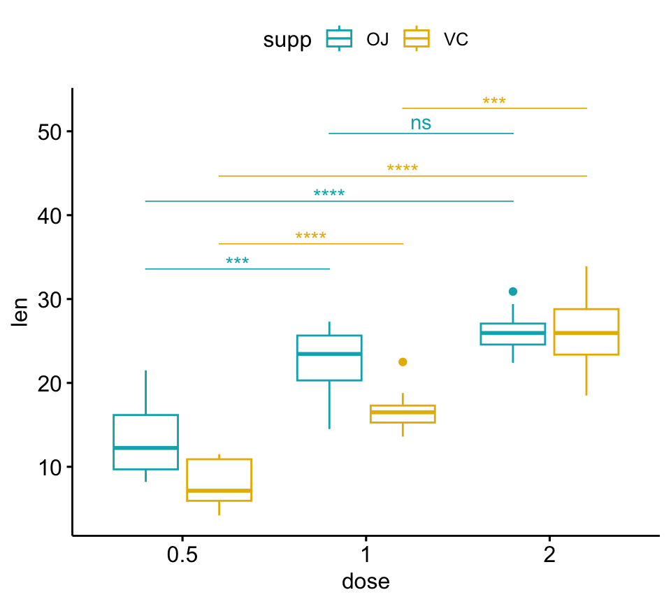
## 3 2 len OJ VC 10 10 -0.0461 14.0 0.964 1 nsGrouped box plots
# Create a box plot
bxp <- ggboxplot(
df, x = "dose", y = "len",
color = "supp", palette = c("#00AFBB", "#E7B800")
)
# Add p-values onto the box plots
stat.test <- stat.test %>%
add_xy_position(x = "dose", dodge = 0.8)
bxp + stat_pvalue_manual(
stat.test, label = "p", tip.length = 0
)
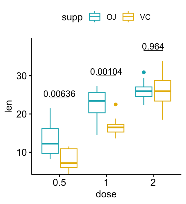
# Add 10% spaces between the p-value labels and the plot border
bxp + stat_pvalue_manual(
stat.test, label = "p", tip.length = 0
) +
scale_y_continuous(expand = expansion(mult = c(0, 0.1)))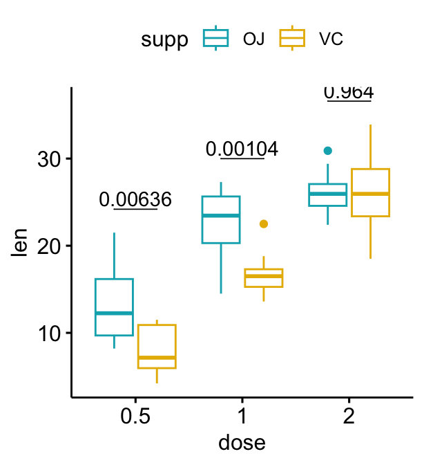
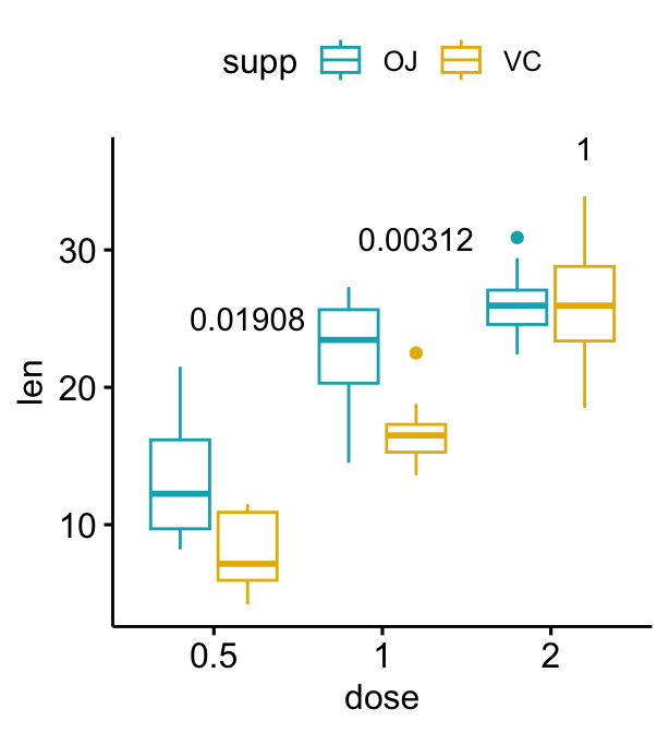
# Use adjusted p-values as labels
# Remove brackets
bxp + stat_pvalue_manual(
stat.test, label = "p.adj", tip.length = 0,
remove.bracket = TRUE
)
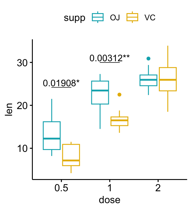
# Show adjusted p-values and significance levels
# Hide ns (non-significant)
bxp + stat_pvalue_manual(
stat.test, label = "{p.adj}{p.adj.signif}",
tip.length = 0, hide.ns = TRUE
)
The following R script create a box plot containing two statistical tests results:
- the above
stat.testcomparing the levels of thesupp(OJvsVC) variable - an additional statistical test (
stat.test2) performing pairwise comparisons between thedoselevels. P-values are automatically adjusted because thedosevariable contains 3 levels.
# Additional statistical test
stat.test2 <- df %>%
  t_test(len ~ dose, p.adjust.method = "bonferroni")
stat.test2
## # A tibble: 3 × 10
## .y. group1 group2 n1 n2 statistic df p p.adj p.adj.signif
## * <chr> <chr> <chr> <int> <int> <dbl> <dbl> <dbl> <dbl> <chr>
## 1 len 0.5 1 20 20 -6.48 38.0 1.27e- 7 3.81e- 7 ****
## 2 len 0.5 2 20 20 -11.8 36.9 4.4 e-14 1.32e-13 ****
## 3 len 1 2 20 20 -4.90 37.1 1.91e- 5 5.73e- 5 ****# Add p-values of `stat.test` and `stat.test2`
# 1. Add stat.test
stat.test <- stat.test %>%
add_xy_position(x = "dose", dodge = 0.8)
bxp.complex <- bxp + stat_pvalue_manual(
stat.test, label = "p", tip.length = 0
)
# 2. Add stat.test2
# Add more space between brackets using `step.increase`
stat.test2 <- stat.test2 %>% add_xy_position(x = "dose")
bxp.complex <- bxp.complex +
stat_pvalue_manual(
stat.test2, label = "p", tip.length = 0.02,
step.increase = 0.05
) +
scale_y_continuous(expand = expansion(mult = c(0.05, 0.1)))
# 3. Display the plot
bxp.complex 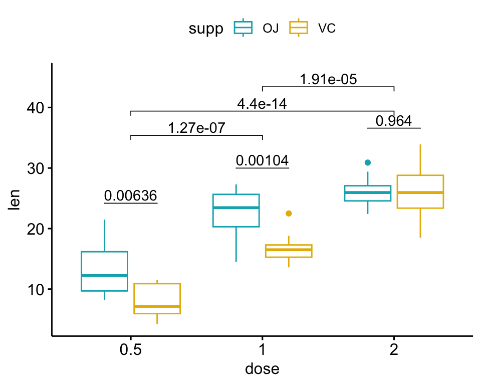
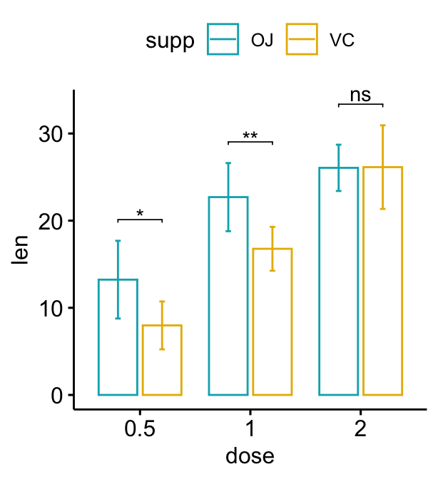
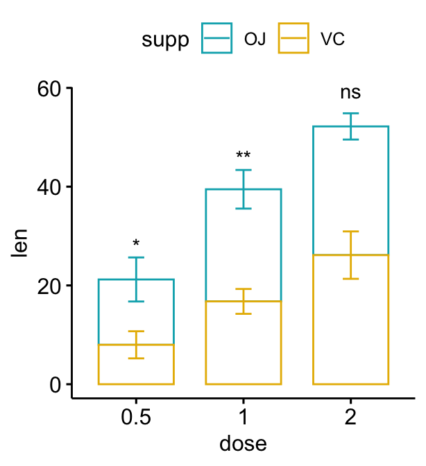
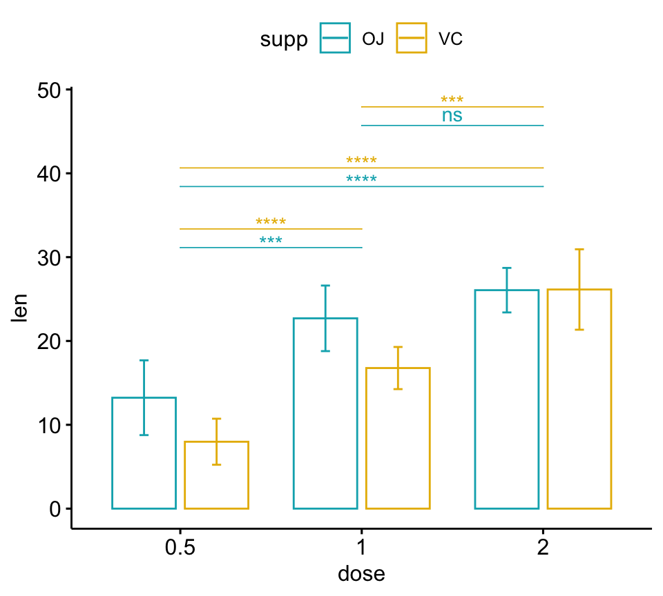
Grouped bar plots
The option add = "mean_sd" is specified in the bar plot function for creating bar plot with error bars (mean +/- SD). You need to specify the same summary statistics function to auto-compute p-value labels positions in add_xy_position() using the option fun.
Dodged bar plots
# Create a bar plot with error bars (mean +/- sd)
bp <- ggbarplot(
df, x = "dose", y = "len", add = "mean_sd",
color= "supp", palette = c("#00AFBB", "#E7B800"),
position = position_dodge(0.8)
)
# Add p-values onto the bar plots
stat.test <- stat.test %>%
add_xy_position(fun = "mean_sd", x = "dose", dodge = 0.8)
bp + stat_pvalue_manual(
stat.test, label = "p.adj.signif", tip.length = 0.01
)
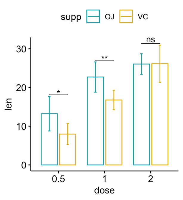
# Move down the brackets using `bracket.nudge.y`
bp + stat_pvalue_manual(
stat.test, label = "p.adj.signif", tip.length = 0,
bracket.nudge.y = -2
)
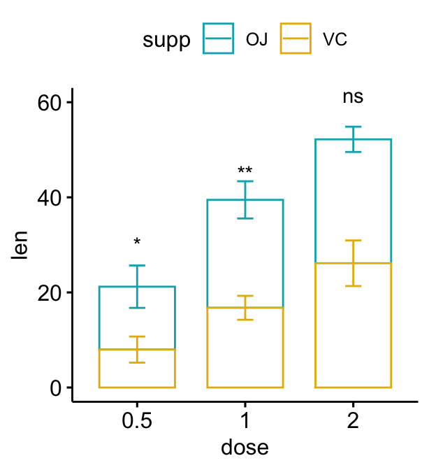
Stacked bar plots
# Create a bar plot with error bars (mean +/- sd)
bp2 <- ggbarplot(
  df, x = "dose", y = "len", add = "mean_sd",
  color = "supp", palette = c("#00AFBB", "#E7B800"),
  position = position_stack()
  )

# Add p-values onto the bar plots
# Specify the p-value y position manually
bp2 + stat_pvalue_manual(
  stat.test,  label = "p.adj.signif", tip.length = 0.01,
  x = "dose", y.position = c(30, 45, 60)
  )

# Auto-compute the p-value y position
# Adjust vertically label positions using vjust
stat.test <- stat.test %>%
  add_xy_position(fun = "mean_sd", x = "dose", stack = TRUE)
bp2 + stat_pvalue_manual(
  stat.test,  label = "p.adj.signif",
  remove.bracket = TRUE, vjust = -0.2
  )
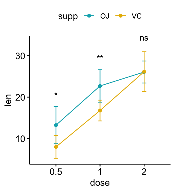
Grouped line plots
# Create a line plot with error bars (mean +/- sd)
lp <- ggline(
df, x = "dose", y = "len", add = "mean_sd",
color = "supp", palette = c("#00AFBB", "#E7B800")
)
# Add p-values onto the line plots
# Remove brackets using linetype = "blank"
stat.test <- stat.test %>%
add_xy_position(fun = "mean_sd", x = "dose")
lp + stat_pvalue_manual(
stat.test, label = "p.adj.signif",
tip.length = 0, linetype = "blank"
)
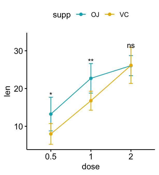
# Move down the significance levels using vjust
lp + stat_pvalue_manual(
stat.test, label = "p.adj.signif",
linetype = "blank", vjust = 2
)
Pairwise comparisons
Statistical tests
Group the data by the supp variable and then perform multiple pairwise comparisons between the levels of the dose variable (0.5, 1 and 2). P-values are adjusted for each group level independently.
pwc <- df %>%
  group_by(supp) %>%
  t_test(len ~ dose, p.adjust.method = "bonferroni")
pwc
## # A tibble: 6 × 11
## supp .y. group1 group2 n1 n2 statistic df p p.adj p.adj.signif
## * <fct> <chr> <chr> <chr> <int> <int> <dbl> <dbl> <dbl> <dbl> <chr>
## 1 OJ len 0.5 1 10 10 -5.05 17.7 0.0000878 0.000263 ***
## 2 OJ len 0.5 2 10 10 -7.82 14.7 0.00000132 0.00000396 ****
## 3 OJ len 1 2 10 10 -2.25 15.8 0.039 0.118 ns
## 4 VC len 0.5 1 10 10 -7.46 17.9 0.000000681 0.00000204 ****
## 5 VC len 0.5 2 10 10 -10.4 14.3 0.0000000468 0.00000014 ****
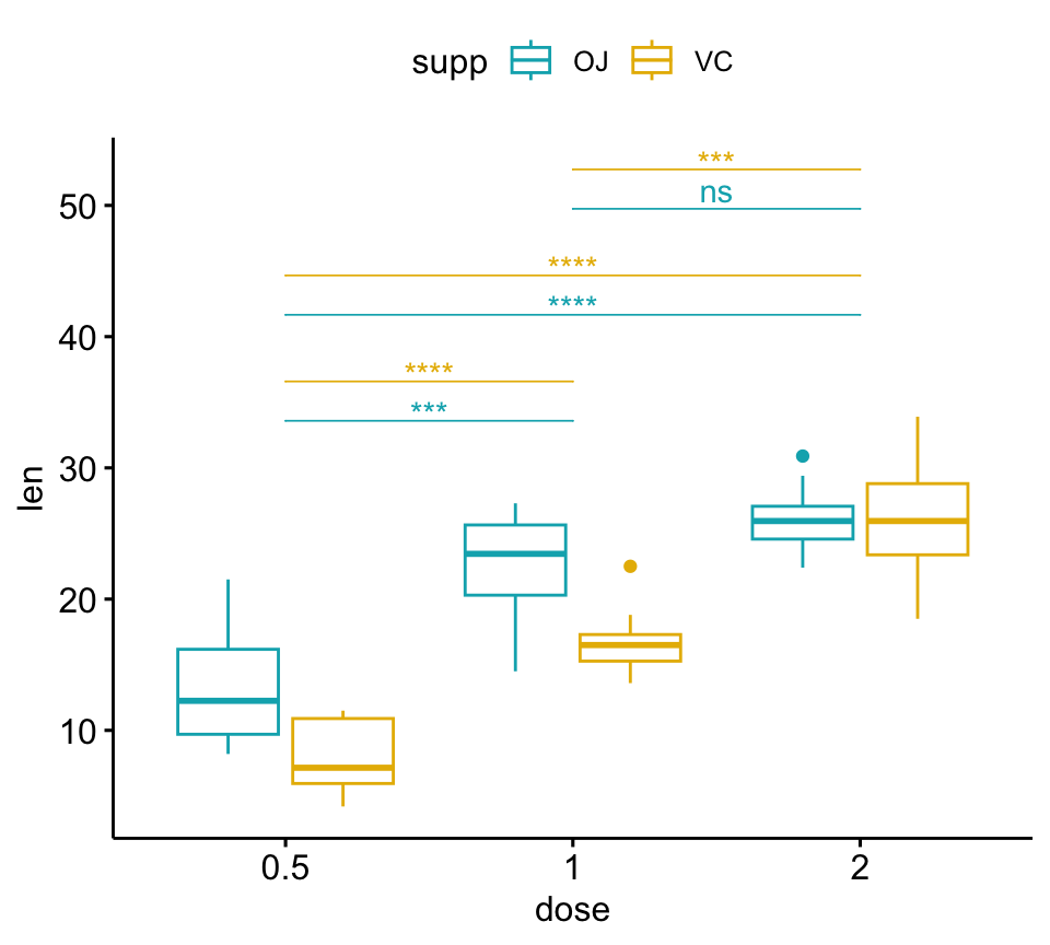
## 6 VC len 1 2 10 10 -5.47 13.6 0.0000916 0.000275 ***Create plots with the pairwise-comparison p-values
The argument step.group.by is used to group the brackets by a variable.
# Box plot
pwc <- pwc %>% add_xy_position(x = "dose")
bxp +
  stat_pvalue_manual(
    pwc, color = "supp", step.group.by = "supp",
    tip.length = 0, step.increase = 0.1
    )
# Adjust brackets x position by the grouping variable
# Specify the group option in add_xy_position()
pwc <- pwc %>% add_xy_position(x = "dose", group = "supp")
bxp +
  stat_pvalue_manual(
    pwc, color = "supp", step.group.by = "supp",
    tip.length = 0, step.increase = 0.1
  )
# Bar plots
pwc <- pwc %>% add_xy_position(x = "dose", fun = "mean_sd", dodge = 0.8)
bp + stat_pvalue_manual(
  pwc, color = "supp", step.group.by = "supp",
  tip.length = 0, step.increase = 0.1
  )
# Line plots
pwc <- pwc %>% add_xy_position(x = "dose", fun = "mean_sd")
lp + stat_pvalue_manual(
  pwc, color = "supp", step.group.by = "supp",
  tip.length = 0, step.increase = 0.1
  )
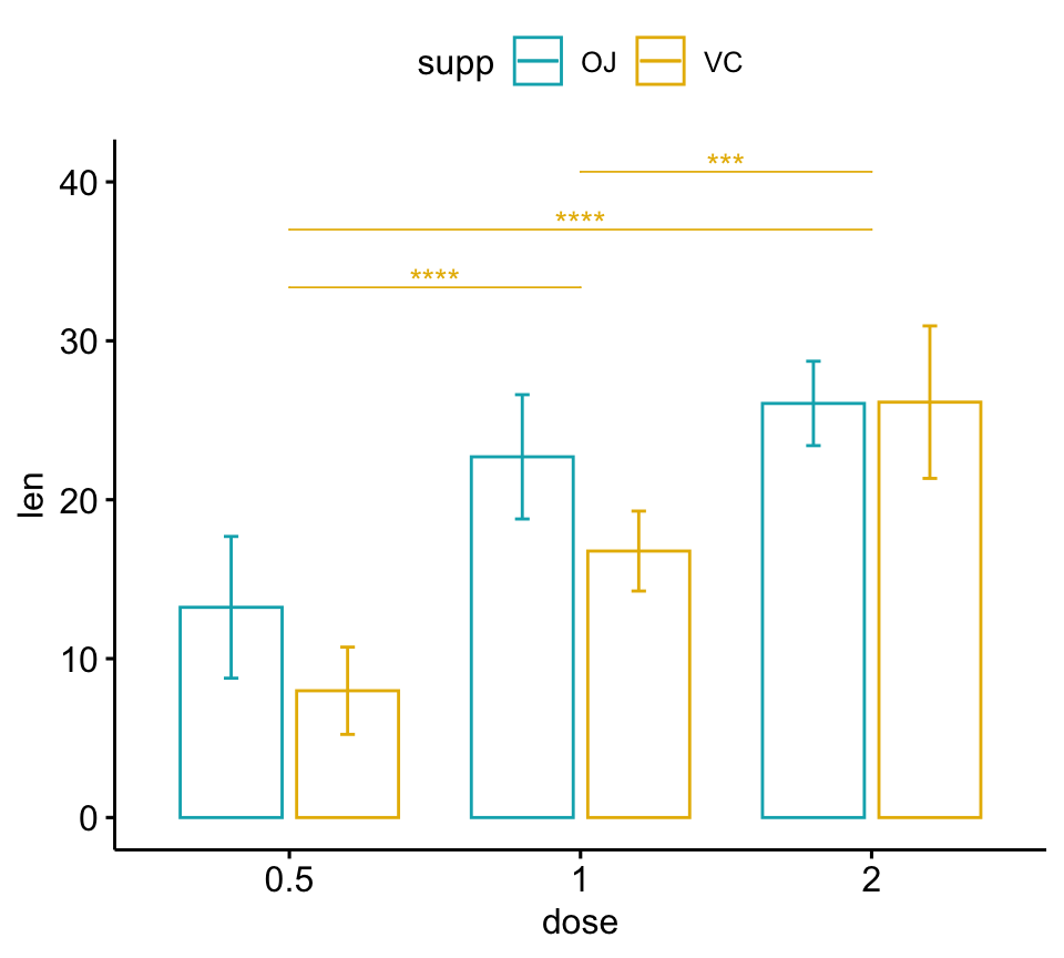
Show the p-values for a subset of comparisons
In the example below, p-values are show for the pairwise-comparisons in the VC group:
# Bar plots (dodged)
# Take a subset of the pairwise comparisons
pwc.filtered <- pwc %>%
  add_xy_position(x = "dose", fun = "mean_sd", dodge = 0.8) %>%
  filter(supp == "VC")
bp +
  stat_pvalue_manual(
    pwc.filtered, color = "supp", step.group.by = "supp",
    tip.length = 0, step.increase = 0
    )
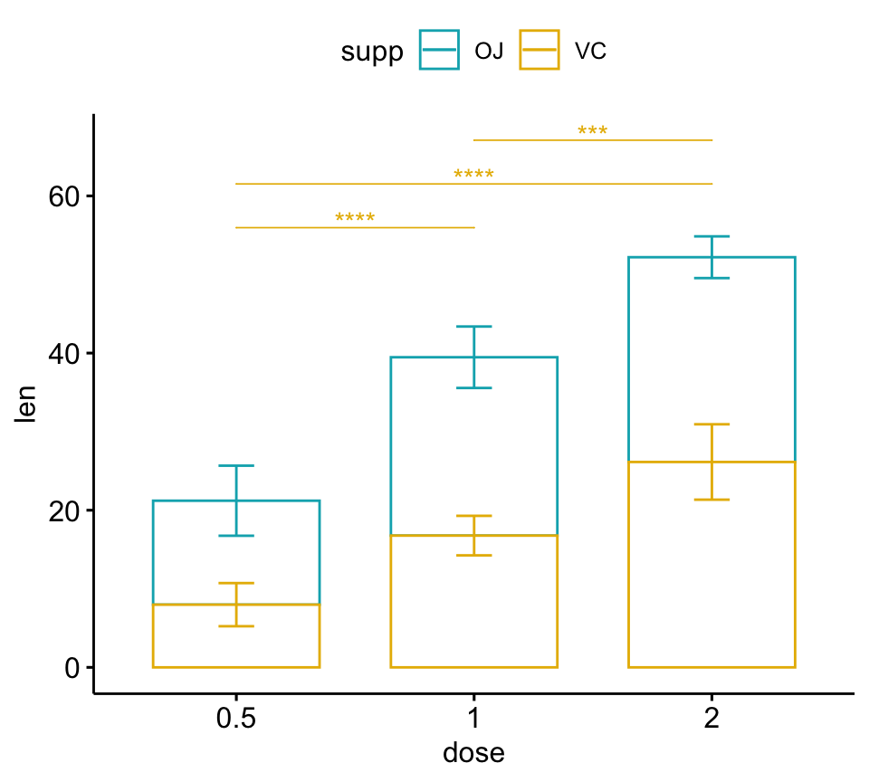
# Bar plots (stacked)
pwc.filtered <- pwc %>%
  add_xy_position(x = "dose", fun = "mean_sd", stack = TRUE) %>%
  filter(supp == "VC")
bp2 +
  stat_pvalue_manual(
    pwc.filtered, color = "supp", step.group.by = "supp",
    tip.length = 0, step.increase = 0.1
    )
Three groups by x position
Simple plots
# Box plots
bxp <- ggboxplot(
df, x = "supp", y = "len", fill = "dose",
palette = "npg"
)
bxp
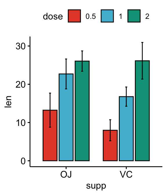
# Bar plots
bp <- ggbarplot(
df, x = "supp", y = "len", fill = "dose",
palette = "npg", add = "mean_sd",
position = position_dodge(0.8)
)
bp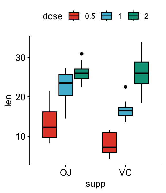
Perform all pairwise comparisons
Group by the supp variable and then perform pairwise comparisons between the levels of dose variable.
Statistical test:
stat.test <- df %>%
  group_by(supp) %>%
  t_test(len ~ dose)
stat.test
## # A tibble: 6 × 11
## supp .y. group1 group2 n1 n2 statistic df p p.adj p.adj.signif
## * <fct> <chr> <chr> <chr> <int> <int> <dbl> <dbl> <dbl> <dbl> <chr>
## 1 OJ len 0.5 1 10 10 -5.05 17.7 0.0000878 0.000176 ***
## 2 OJ len 0.5 2 10 10 -7.82 14.7 0.00000132 0.00000396 ****
## 3 OJ len 1 2 10 10 -2.25 15.8 0.039 0.039 *
## 4 VC len 0.5 1 10 10 -7.46 17.9 0.000000681 0.00000136 ****
## 5 VC len 0.5 2 10 10 -10.4 14.3 0.0000000468 0.00000014 ****
## 6 VC len 1 2 10 10 -5.47 13.6 0.0000916 0.0000916 ****Add the p-values onto the plots:
- The argument
bracket.nudge.yis used to move down the brackets. - The ggplot2 function
scale_y_continuous(expand = expansion(mult = c(0, 0.1)))is used to add more spaces between labels and the plot top border
# Box plots with p-values
stat.test <- stat.test %>%
  add_xy_position(x = "supp", dodge = 0.8)
bxp +
  stat_pvalue_manual(
    stat.test, label = "p.adj", tip.length = 0.01,
    bracket.nudge.y = -2
    ) +
  scale_y_continuous(expand = expansion(mult = c(0, 0.1)))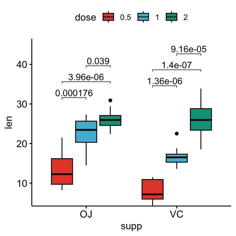
# Bar plots with p-values
stat.test <- stat.test %>%
  add_xy_position(x = "supp", fun = "mean_sd", dodge = 0.8)
bp +
  stat_pvalue_manual(
    stat.test, label = "p.adj", tip.length = 0.01,
    bracket.nudge.y = -2
    ) +
  scale_y_continuous(expand = expansion(mult = c(0, 0.1)))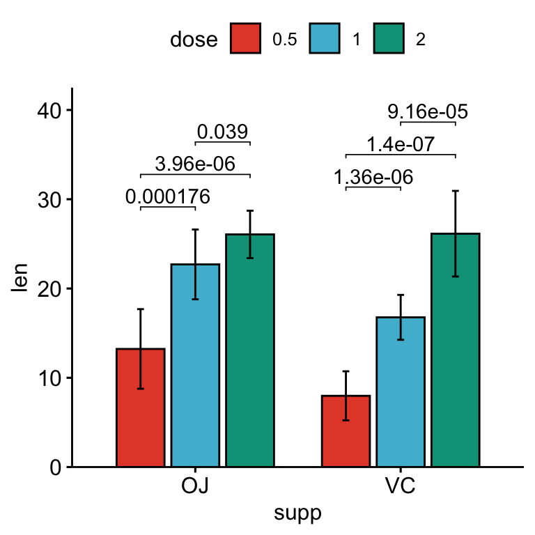
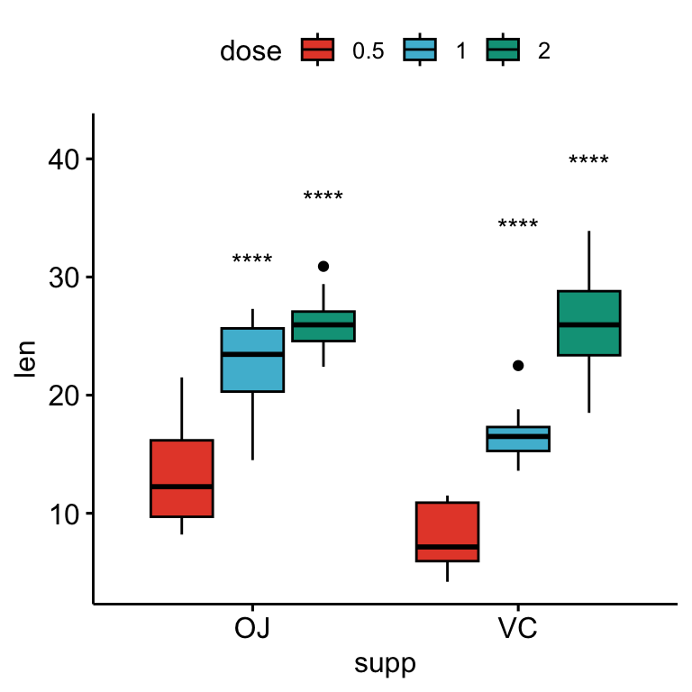
Pairwise comparisons against a reference group
Statistical tests:
stat.test <- df %>%
  group_by(supp) %>%
  t_test(len ~ dose, ref.group = "0.5")
stat.test
## # A tibble: 4 × 11
## supp .y. group1 group2 n1 n2 statistic df p p.adj p.adj.signif
## * <fct> <chr> <chr> <chr> <int> <int> <dbl> <dbl> <dbl> <dbl> <chr>
## 1 OJ len 0.5 1 10 10 -5.05 17.7 0.0000878 0.0000878 ****
## 2 OJ len 0.5 2 10 10 -7.82 14.7 0.00000132 0.00000264 ****
## 3 VC len 0.5 1 10 10 -7.46 17.9 0.000000681 0.000000681 ****
## 4 VC len 0.5 2 10 10 -10.4 14.3 0.0000000468 0.0000000936 ****# Box plots with p-values
stat.test <- stat.test %>%
add_xy_position(x = "supp", dodge = 0.8)
bxp +
stat_pvalue_manual(
stat.test, label = "p.adj", tip.length = 0.01,
bracket.nudge.y = -2
) +
scale_y_continuous(expand = expansion(mult = c(0, 0.1)))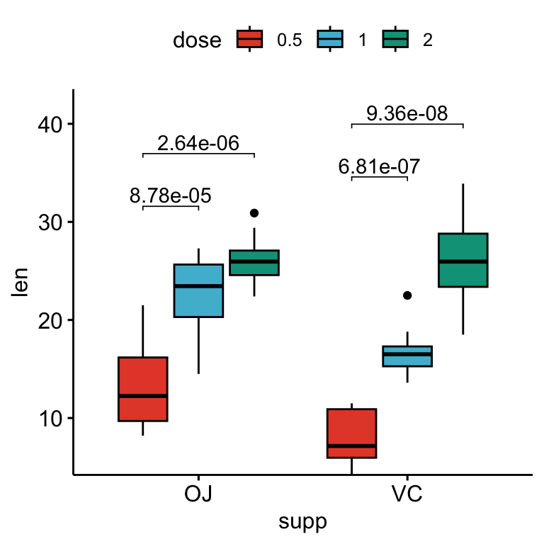
# Show only significance levels
# Move down significance symbols using vjust
bxp + stat_pvalue_manual(
  stat.test, x = "supp",  label = "p.adj.signif",
  tip.length = 0.01, vjust = 2
  )
# Bar plots with p-values
stat.test <- stat.test %>%
  add_xy_position(x = "supp", fun = "mean_sd", dodge = 0.8)
bp +
  stat_pvalue_manual(
    stat.test, label = "p.adj", tip.length = 0.01,
    bracket.nudge.y = -2
    ) +
  scale_y_continuous(expand = expansion(mult = c(0, 0.1)))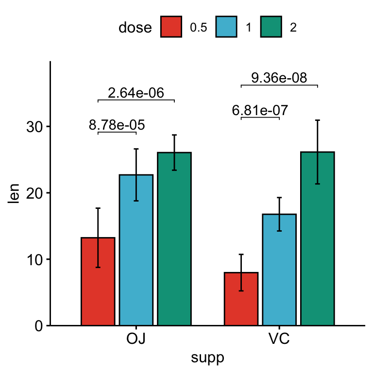
Conclusion
This article describes how to add p-values onto grouped ggplots, such as box plots, bar plots and line plots. See other related frequently questions: ggpubr FAQ.
Recommended for you
This section contains best data science and self-development resources to help you on your path.
Books - Data Science
Our Books
- Practical Guide to Cluster Analysis in R by A. Kassambara (Datanovia)
- Practical Guide To Principal Component Methods in R by A. Kassambara (Datanovia)
- Machine Learning Essentials: Practical Guide in R by A. Kassambara (Datanovia)
- R Graphics Essentials for Great Data Visualization by A. Kassambara (Datanovia)
- GGPlot2 Essentials for Great Data Visualization in R by A. Kassambara (Datanovia)
- Network Analysis and Visualization in R by A. Kassambara (Datanovia)
- Practical Statistics in R for Comparing Groups: Numerical Variables by A. Kassambara (Datanovia)
- Inter-Rater Reliability Essentials: Practical Guide in R by A. Kassambara (Datanovia)
Others
- R for Data Science: Import, Tidy, Transform, Visualize, and Model Data by Hadley Wickham & Garrett Grolemund
- Hands-On Machine Learning with Scikit-Learn, Keras, and TensorFlow: Concepts, Tools, and Techniques to Build Intelligent Systems by Aurelien Géron
- Practical Statistics for Data Scientists: 50 Essential Concepts by Peter Bruce & Andrew Bruce
- Hands-On Programming with R: Write Your Own Functions And Simulations by Garrett Grolemund & Hadley Wickham
- An Introduction to Statistical Learning: with Applications in R by Gareth James et al.
- Deep Learning with R by François Chollet & J.J. Allaire
- Deep Learning with Python by François Chollet
Version:
 Français


Outstanding blog post, thank you.
Just a comment that I think the convenience function `expansion()` inside ggplot2 may have been deprecated; replaced with the equivalent function expand_scale()
Thank you for the positive feedback. In the latest CRAN version of ggplot2 (v3.3.0) it’s the opposite that holds TRUE. `expand_scale()` is deprecated but not `expansion()`.
First, thanks a lot for great jobs, I’m new at this job and I can do some analysis because of you and there is amazing report graphs.
But, unfortunately I have problem for one group repeated actions. I tried a lot (with “https://www.datanovia.com/en/blog/how-to-add-p-values-onto-a-grouped-ggplot-using-the-ggpubr-r-package/” to show p values on boxplot like in this page, ..whenever I tried to fix to “one group” for my study..I couldnt achieved… Could you share a link for this?
I think, It would be great if there are different more representations (ggplots , ggviolin etc.) of repetitive measurements in this “”https://www.datanovia.com/en/lessons/repeated-measures-anova-in-r/ “” link as well.
thanks again.
Hi,
If I understood correctly, the issue is about displaying the p-values of one-way repeated measures ANOVA, isn’t it? Please provide a demo data, demo graph or a reproducible script to help me understanding the issue. You can publish here a reproducible script here using the pubr package or on github (https://github.com/kassambara/ggpubr)
Yes it is..just shared..skipped some steps (normality check , qqplot etc.) tried show 2 way..Issue 1 and 2..
“””https://github.com/kassambara/ggpubr/compare/master…berman954:patch-1″”
In your example, the following R code should work for adding p-values on the box-plot:
I need to work more about it. Thanks a lot for your help!
Note: If someone like me is trying to do this new job, I suggest you follow the comments above. In my opinion, the simplest and effective “one/two way repeated measures ANOVA” analysis among others.
“https://www.datanovia.com/en/lessons/repeated-measures-anova-in-r/”
Hello, Fantastic tutorial. Is there a way to remove ns from the plots? I have applied the hide.ns function as detailed in your methods. However, when I apply it to multiple comparisons it does hide the ns but leaves a big gap between the significant numbers. Is there a way to remove the ns? Thank you
I would really like to Appreciate your commitments to let others attracted to R, Very kindly keep it up, sharing is happiness!!
Hi. Thank you so much for this tutorial! I am quite new to R and I have some data that I put into boxplots and added the p-values. I used the code you used for the pairwise comparison but my p-values seems to have shifted to the right. Can you please help me?
Dear Dr. Kassambara,
Thank you for the great software for creating scientific charts.
However, I have a problem with creating a line graph showing two series of results, where I compare Defensemens and Forwards for Hrmin and Hrpeak, further grouped by the variable “Protocol”. Unfortunately, the code does not work despite entering “combine = T”. Could I please help me solve this problem?
Best wishes,
Ark Sta
library(ggpubr)
#> Ładowanie wymaganego pakietu: ggplot2
library(rstatix)
#>
#> Dołączanie pakietu: ‘rstatix’
#> Następujący obiekt został zakryty z ‘package:stats’:
#>
#> filter
library(tidyverse)
df <- data.frame(
stringsAsFactors = FALSE,
ID = c(1L,2L,3L,4L,5L,6L,7L,8L,
9L,10L,11L,12L,13L,14L,1L,2L,3L,4L,5L,6L,7L,
8L,9L,10L,11L,12L,13L,14L,1L,2L,3L,4L,5L,6L,
7L,8L,9L,10L,11L,12L,13L,14L,1L,2L,3L,4L,5L,
6L,7L,8L,9L,10L,11L,12L,13L,14L,1L,2L,3L,4L,
5L,6L,7L,8L,9L,10L,11L,12L,13L,14L,1L,2L,3L,
4L,5L,6L,7L,8L,9L,10L,11L,12L,13L,14L),
Protocol = c("RSSA-2","RSSA-2","RSSA-2",
"RSSA-2","RSSA-2","RSSA-2","RSSA-2","RSSA-2","RSSA-2",
"RSSA-2","RSSA-2","RSSA-2","RSSA-2","RSSA-2",
"RSSA-3","RSSA-3","RSSA-3","RSSA-3","RSSA-3","RSSA-3",
"RSSA-3","RSSA-3","RSSA-3","RSSA-3","RSSA-3","RSSA-3",
"RSSA-3","RSSA-3","RSSA-2","RSSA-2","RSSA-2",
"RSSA-2","RSSA-2","RSSA-2","RSSA-2","RSSA-2","RSSA-2",
"RSSA-2","RSSA-2","RSSA-2","RSSA-2","RSSA-2","RSSA-3",
"RSSA-3","RSSA-3","RSSA-3","RSSA-3","RSSA-3",
"RSSA-3","RSSA-3","RSSA-3","RSSA-3","RSSA-3","RSSA-3",
"RSSA-3","RSSA-3","RSSA-2","RSSA-2","RSSA-2","RSSA-2",
"RSSA-2","RSSA-2","RSSA-2","RSSA-2","RSSA-2","RSSA-2",
"RSSA-2","RSSA-2","RSSA-2","RSSA-2","RSSA-3",
"RSSA-3","RSSA-3","RSSA-3","RSSA-3","RSSA-3","RSSA-3",
"RSSA-3","RSSA-3","RSSA-3","RSSA-3","RSSA-3","RSSA-3",
"RSSA-3"),
Position = c("Forwards","Forwards",
"Forwards","Forwards","Forwards","Forwards","Forwards",
"Defensemen","Defensemen","Defensemen","Defensemen",
"Defensemen","Defensemen","Defensemen","Forwards",
"Forwards","Forwards","Forwards","Forwards","Forwards",
"Forwards","Defensemen","Defensemen","Defensemen",
"Defensemen","Defensemen","Defensemen","Defensemen",
"Forwards","Forwards","Forwards","Forwards","Forwards",
"Forwards","Forwards","Defensemen","Defensemen",
"Defensemen","Defensemen","Defensemen","Defensemen","Defensemen",
"Forwards","Forwards","Forwards","Forwards",
"Forwards","Forwards","Forwards","Defensemen","Defensemen",
"Defensemen","Defensemen","Defensemen","Defensemen",
"Defensemen","Forwards","Forwards","Forwards",
"Forwards","Forwards","Forwards","Forwards","Defensemen",
"Defensemen","Defensemen","Defensemen","Defensemen",
"Defensemen","Defensemen","Forwards","Forwards",
"Forwards","Forwards","Forwards","Forwards","Forwards",
"Defensemen","Defensemen","Defensemen","Defensemen",
"Defensemen","Defensemen","Defensemen"),
SET = c("SET-1","SET-1","SET-1",
"SET-1","SET-1","SET-1","SET-1","SET-1","SET-1","SET-1",
"SET-1","SET-1","SET-1","SET-1","SET-1","SET-1",
"SET-1","SET-1","SET-1","SET-1","SET-1","SET-1",
"SET-1","SET-1","SET-1","SET-1","SET-1","SET-1","SET-2",
"SET-2","SET-2","SET-2","SET-2","SET-2","SET-2",
"SET-2","SET-2","SET-2","SET-2","SET-2","SET-2",
"SET-2","SET-2","SET-2","SET-2","SET-2","SET-2","SET-2",
"SET-2","SET-2","SET-2","SET-2","SET-2","SET-2",
"SET-2","SET-2","SET-3","SET-3","SET-3","SET-3",
"SET-3","SET-3","SET-3","SET-3","SET-3","SET-3","SET-3",
"SET-3","SET-3","SET-3","SET-3","SET-3","SET-3",
"SET-3","SET-3","SET-3","SET-3","SET-3","SET-3",
"SET-3","SET-3","SET-3","SET-3","SET-3"),
Hrmin = c(58.9,60,48.2,62.9,47.9,
62.6,75.1,59.4,67.7,61.1,65.6,67.7,80.6,55.1,61.6,
61.6,49.2,59.8,59.3,64.7,68.9,63.4,59.5,57,62.6,
61,72,67.9,77.3,78.4,65.3,70.1,72.7,67.4,64.2,
78.7,81.5,76.2,78.5,70.8,84.9,58.7,68.6,77.4,
59.1,65.5,74.2,71.7,74.6,62.9,66.7,65.8,71.8,64.1,
75.8,72.4,80.5,82.1,67.4,78.9,74.2,70.6,68.4,
80.7,82.1,77.7,84.6,70.8,84.9,69.9,74.6,75.3,64.8,
65.5,73.7,68.4,74.1,71.3,67.7,65.8,75.9,56.9,78,
80.1),
Hrpeak = c(87.6,84.7,83.9,89.2,79.9,
85.6,96.9,93.1,90.8,89.6,94.9,87.7,96.2,89.8,88.1,
90,84.5,92.8,88.1,92,94.8,88.1,88.2,89.6,85.1,
83.6,94.1,93.4,90.3,92.1,87.6,91.2,85.1,87.7,
90.2,90.6,93.8,92.7,95.4,89.7,97.8,92.3,91.4,91.6,
89.1,94.8,90.2,94.1,94.8,89.1,90.3,91.2,94.9,
87.2,95.7,94.4,90.3,91.1,90.2,94.8,88.1,91.4,98.4,
89.1,93.8,93.8,94.9,90.8,97.8,92.3,93,91.6,91.2,
94.8,89.7,96.3,96.4,90.6,91.3,92.7,94.9,87.2,
95.7,94.4))
stat.test_1 %
group_by(Protocol, SET) %>%
tukey_hsd(Hrpeak ~ Position) %>%
adjust_pvalue(method = “bonferroni”) %>%
add_significance(“p.adj”)
stat.test_1 % add_xy_position(x = “SET”, fun = “mean_ci”, dodge = 0.8)
stat.test_1$p.format <- p_format(stat.test_1$p.adj, accuracy = 0.001, leading.zero = TRUE)
stat.test_2 %
group_by(Protocol, SET) %>%
tukey_hsd(Hrmin ~ Position) %>%
adjust_pvalue(method = “bonferroni”) %>%
add_significance(“p.adj”)
stat.test_2 % add_xy_position(x = “SET”, fun = “mean_ci”, dodge = 0.8)
stat.test_2$p.format <- p_format(stat.test_2$p.adj, accuracy = 0.001, leading.zero = TRUE)
ggline(
df, x = "SET", y = c("Hrpeak", "Hrmin"), combine = T, merge = F, add = "mean_ci", add.params = list(width = .5),
color = "Position", palette = c("#FF6347", "#4787FF"), position = position_dodge(0.5)) +
facet_wrap(~Protocol, labeller = label_parsed) +
labs(x = "Sets of RSSA", y = "Percentage of Maximum Heart Rate (%)") +
stat_pvalue_manual(stat.test_1, label = "{p.format}{p.adj.signif}", hide.ns = FALSE, tip.length = 0) +
stat_pvalue_manual(stat.test_2, label = "{p.format}{p.adj.signif}", hide.ns = FALSE, tip.length = 0) +
scale_y_continuous(limits = c(45, 100), breaks=seq(50,100,10), expand = expansion(mult = c(0.05, 0.1)))
Sorry, but in the stat.test 1 and 2 part of the code the operator %>% was not copied. Therefore, I allow myself to paste again…
stat.test_1 %
group_by(Protocol, SET) %>%
tukey_hsd(Hrpeak ~ Position) %>%
adjust_pvalue(method = “bonferroni”) %>%
add_significance(“p.adj”)
stat.test_1 % add_xy_position(x = “SET”, fun = “mean_ci”, dodge = 0.8)
stat.test_1$p.format <- p_format(stat.test_1$p.adj, accuracy = 0.001, leading.zero = TRUE)
stat.test_2 %
group_by(Protocol, SET) %>%
tukey_hsd(Hrmin ~ Position) %>%
adjust_pvalue(method = “bonferroni”) %>%
add_significance(“p.adj”)
stat.test_2 % add_xy_position(x = “SET”, fun = “mean_ci”, dodge = 0.8)
stat.test_2$p.format <- p_format(stat.test_2$p.adj, accuracy = 0.001, leading.zero = TRUE)
Hi,
Is there a way to adjust the cutpoints of significance?
Using something like :
symnum.args=list(cutpoints = c(0, 0.0001, 0.001, 0.01, 0.05,0.1, 1), symbols = c(“****”, “***”, “**”, “*”,”.”, “ns”)))
Thanks!
for the example where you create a box plot containing two statistical tests results, is it possible to complete stat.test2 by just comparing the doses of one factor of supp, so just OJ for example?
Hello, very nice tutorial. How can display the standard error instead of mean of sd?
Thank you so much
Thanks for your explicit tutorial~~ I ran my data as your protocol, but there are some error happened, like “Error in FUN(X[[i]], …) : object ‘cond’ not found”, in which “cond”means the group I wanna do t test. I do not know what is wrong going here~ Can you help me ?
t_test %
group_by(choice,stimu)%>%
t_test(frequency ~ cond, paired = TRUE,p.adjust.method = “bonferroni”)%>%
add_significance()
t_test% add_xy_position(x = “choice”,
fun = “mean_sd”, dodge = 0.8)
ggplot(choice_count,aes(x=choice, y = frequency, fill = cond, color = cond))+
facet_grid(. ~ stimu)+
geom_boxplot(alpha = 0.7)+
stat_compare_means(method = ‘anova’, label.y = 28)+
stat_pvalue_manual(t_test, label = “p.adj.signif”, tip.length = 0.01)