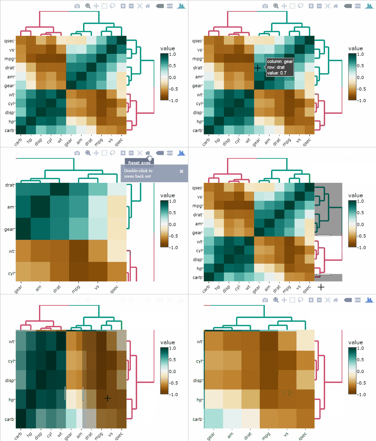
Data normalization methods are used to make variables, measured in different scales, have comparable values. This preprocessing steps is important for clustering and heatmap visualization, principal component analysis and other machine learning algorithms based on distance measures.
This article describes the following data rescaling approaches:
- Standard scaling or standardization
- Normalization or Min-Max scaling
- Percentile transformation
Codes will be provided to demonstrate how to standardize, normalize and percentilize data in R. The R package heatmaply contains helper functions for normalizing and visualizing data as interactive heatmap.
Contents:
Prerequisites
The heatmaply R package will be used to interactively visualize the data before and after transformation.
Install the packages using install.packages("heatmaply"), then load it as follow:
library(heatmaply)Heatmap of the raw data
heatmaply(
  mtcars,
  xlab = "Features",
  ylab = "Cars",
  main = "Raw data"
)Standard scaling
Standard scaling, also known as standardization or Z-score normalization, consists of subtracting the mean and divide by the standard deviation. In such a case, each value would reflect the distance from the mean in units of standard deviation.
If we would assume all variables come from some normal distribution, then scaling would bring them all close to the standard normal distribution. The resulting distribution has a mean of 0 and a standard deviation of 1.
Standard scaling formula:
\[Transformed.Values = \frac{Values - Mean}{Standard.Deviation}\]
An alternative to standardization is the mean normalization, which resulting distribution will have between -1 and 1 with mean = 0.
Mean normalization formula:
\[Transformed.Values = \frac{Values - Mean}{Maximum - Minimum}\]
Standardization and Mean Normalization can be used for algorithms that assumes zero centric data like Principal Component Analysis(PCA).
The following R code standardizes the mtcars data set and creates a heatmap:
heatmaply(
  scale(mtcars),
  xlab = "Features",
  ylab = "Cars",
  main = "Data Scaling"
)Normalization
When variables in the data comes from possibly different (and non-normal) distributions, other transformations may be in order. Another possibility is to normalize the variables to brings data to the 0 to 1 scale by subtracting the minimum and dividing by the maximum of all observations.
This preserves the shape of each variable’s distribution while making them easily comparable on the same “scale”.
Formula to normalize data between 0 and 1 :
\[Transformed.Values = \frac{Values - Minimum}{Maximum - Minimum}\]
Formula to rescale the data between an arbitrary set of values [a, b]:
\[
Transformed.Values = a + \frac{(Values - Minimum)(b-a)}{Maximum - Minimum}
\]
where a,b are the min-max values.
Normalize data in R. Using the Min-Max normalization function on mtcars data easily reveals columns with only two (am, vs) or three (gear, cyl) variables compared with variables that have a higher resolution of possible values:
heatmaply(
  normalize(mtcars),
  xlab = "Features",
  ylab = "Cars",
  main = "Data Normalization"
)Percentile transformation
An alternative to normalize is the percentize function. This is similar to ranking the variables, but instead of keeping the rank values, divide them by the maximal rank. This is done by using the ecdf of the variables on their own values, bringing each value to its empirical percentile. The benefit of the percentize function is that each value has a relatively clear interpretation, it is the percent of observations with that value or below it.
heatmaply(
  percentize(mtcars),
  xlab = "Features",
  ylab = "Cars",
  main = "Percentile Transformation"
)Notice that for binary variables (0 and 1), the percentile transformation will turn all 0 values to their proportion and all 1 values will remain 1. This means the transformation is not symmetric for 0 and 1. Hence, if scaling for clustering, it might be better to use rank for dealing with tie values (if no ties are present, then percentize will perform similarly to rank).
References
Recommended for you
This section contains best data science and self-development resources to help you on your path.
Books - Data Science
Our Books
- Practical Guide to Cluster Analysis in R by A. Kassambara (Datanovia)
- Practical Guide To Principal Component Methods in R by A. Kassambara (Datanovia)
- Machine Learning Essentials: Practical Guide in R by A. Kassambara (Datanovia)
- R Graphics Essentials for Great Data Visualization by A. Kassambara (Datanovia)
- GGPlot2 Essentials for Great Data Visualization in R by A. Kassambara (Datanovia)
- Network Analysis and Visualization in R by A. Kassambara (Datanovia)
- Practical Statistics in R for Comparing Groups: Numerical Variables by A. Kassambara (Datanovia)
- Inter-Rater Reliability Essentials: Practical Guide in R by A. Kassambara (Datanovia)
Others
- R for Data Science: Import, Tidy, Transform, Visualize, and Model Data by Hadley Wickham & Garrett Grolemund
- Hands-On Machine Learning with Scikit-Learn, Keras, and TensorFlow: Concepts, Tools, and Techniques to Build Intelligent Systems by Aurelien Géron
- Practical Statistics for Data Scientists: 50 Essential Concepts by Peter Bruce & Andrew Bruce
- Hands-On Programming with R: Write Your Own Functions And Simulations by Garrett Grolemund & Hadley Wickham
- An Introduction to Statistical Learning: with Applications in R by Gareth James et al.
- Deep Learning with R by François Chollet & J.J. Allaire
- Deep Learning with Python by François Chollet
Version:
 Français


Hi Kassambara,
I absolutely adore your articles. Thank you so so much for your amazing work. Super helpful!
I always had a question in regards scaling/normalizing data.
Depending on the method you use the clustering of the elements change. Sometimes it can change quite a lot. Then, how do you know which dendrogram is correct? Are all correct? Because, I am biologist and the interpretation of the data can vary substantially.
Again, thank you for your great contribution and help.
Jaz (Australia)
Thank you Jazmina for your positive feedback, highly appreciated!
Standardization or Min-Max normalization?. There is no obvious answer to this question: it really depends on the application.
For example, in clustering analyses, standardization may be especially crucial in order to compare similarities between features based on certain distance measures.
Another example is the Principal Component Analysis, where we usually prefer standardization over Min-Max scaling, since we are interested in the components that maximize the variance.
In highthroughput gene expression data analyses,people tends to perform clustering on the standardized data (
scale(log2(expression_data)))A popular application of Min-Max scaling (or normalization) is image processing, where pixel intensities have to be normalized to fit within a certain range (i.e., 0 to 255 for the RGB color range). Also, typical neural network algorithm require data that on a 0-1 scale.