Mixed ANOVA is used to compare the means of groups cross-classified by two different types of factor variables, including:
- between-subjects factors, which have independent categories (e.g., gender: male/female)
- within-subjects factors, which have related categories also known as repeated measures (e.g., time: before/after treatment).
The mixed ANOVA test is also referred as mixed design ANOVA and mixed measures ANOVA.
This chapter describes different types of mixed ANOVA, including:
- two-way mixed ANOVA, used to compare the means of groups cross-classified by two independent categorical variables, including one between-subjects and one within-subjects factors.
- three-way mixed ANOVA, used to evaluate if there is a three-way interaction between three independent variables, including between-subjects and within-subjects factors. You can have two different designs for three-way mixed ANOVA:
- one between-subjects factor and two within-subjects factors
- two between-subjects factor and one within-subjects factor
You will learn how to:
- Compute and interpret the different mixed ANOVA tests in R.
- Check mixed ANOVA test assumptions
- Perform post-hoc tests, multiple pairwise comparisons between groups to identify which groups are different
- Visualize the data using box plots, add ANOVA and pairwise comparisons p-values to the plot
Contents:
Related Book
Practical Statistics in R II - Comparing Groups: Numerical VariablesAssumptions
The mixed ANOVA makes the following assumptions about the data:
- No significant outliers in any cell of the design. This can be checked by visualizing the data using box plot methods and by using the function
identify_outliers()[rstatix package]. - Normality: the outcome (or dependent) variable should be approximately normally distributed in each cell of the design. This can be checked using the Shapiro-Wilk normality test (
shapiro_test()[rstatix]) or by visual inspection using QQ plot (ggqqplot()[ggpubr package]). - Homogeneity of variances: the variance of the outcome variable should be equal between the groups of the between-subjects factors. This can be assessed using the Levene’s test for equality of variances (
levene_test()[rstatix]). - Assumption of sphericity: the variance of the differences between within-subjects groups should be equal. This can be checked using the Mauchly’s test of sphericity, which is automatically reported when using the
anova_test()R function. - Homogeneity of covariances tested by Box’s M. The covariance matrices should be equal across the cells formed by the between-subjects factors.
Before computing mixed ANOVA test, you need to perform some preliminary tests to check if the assumptions are met.
Prerequisites
Make sure that you have installed the following R packages:
tidyversefor data manipulation and visualizationggpubrfor creating easily publication ready plotsrstatixprovides pipe-friendly R functions for easy statistical analysesdatarium: contains required data sets for this chapter
Start by loading the following R packages:
library(tidyverse)
library(ggpubr)
library(rstatix)
Key R functions:
anova_test()[rstatix package], a wrapper aroundcar::Anova()for making easy the computation of repeated measures ANOVA. Key arguments for performing repeated measures ANOVA:data: data framedv: (numeric) the dependent (or outcome) variable name.wid: variable name specifying the case/sample identifier.between: between-subjects factor or grouping variablewithin: within-subjects factor or grouping variable
get_anova_table()[rstatix package]. Extracts the ANOVA table from the output ofanova_test(). It returns ANOVA table that is automatically corrected for eventual deviation from the sphericity assumption. The default is to apply automatically the Greenhouse-Geisser sphericity correction to only within-subject factors violating the sphericity assumption (i.e., Mauchly’s test p-value is significant, p <= 0.05). Read more in Chapter @ref(mauchly-s-test-of-sphericity-in-r).
Two-way mixed ANOVA
Data preparation
We’ll use the anxiety dataset [in the datarium package], which contains the anxiety score, measured at three time points (t1, t2 and t3), of three groups of individuals practicing physical exercises at different levels (grp1: basal, grp2: moderate and grp3: high)
Two-way mixed ANOVA can be used to evaluate if there is interaction between group and time in explaining the anxiety score.
Load and show one random row by group:
# Wide format
set.seed(123)
data("anxiety", package = "datarium")
anxiety %>% sample_n_by(group, size = 1)
## # A tibble: 3 x 5
## id group t1 t2 t3
## <fct> <fct> <dbl> <dbl> <dbl>
## 1 5 grp1 16.5 15.8 15.7
## 2 27 grp2 17.8 17.7 16.9
## 3 37 grp3 17.1 15.6 14.3# Gather the columns t1, t2 and t3 into long format.
# Convert id and time into factor variables
anxiety <- anxiety %>%
gather(key = "time", value = "score", t1, t2, t3) %>%
convert_as_factor(id, time)
# Inspect some random rows of the data by groups
set.seed(123)
anxiety %>% sample_n_by(group, time, size = 1)## # A tibble: 9 x 4
## id group time score
## <fct> <fct> <fct> <dbl>
## 1 5 grp1 t1 16.5
## 2 12 grp1 t2 17.7
## 3 7 grp1 t3 16.5
## 4 29 grp2 t1 18.4
## 5 30 grp2 t2 18.9
## 6 16 grp2 t3 12.7
## # … with 3 more rowsSummary statistics
Group the data by time and group, and then compute some summary statistics of the score variable: mean and sd (standard deviation)
anxiety %>%
  group_by(time, group) %>%
  get_summary_stats(score, type = "mean_sd")
## # A tibble: 9 x 6
## group time variable n mean sd
## <fct> <fct> <chr> <dbl> <dbl> <dbl>
## 1 grp1 t1 score 15 17.1 1.63
## 2 grp2 t1 score 15 16.6 1.57
## 3 grp3 t1 score 15 17.0 1.32
## 4 grp1 t2 score 15 16.9 1.70
## 5 grp2 t2 score 15 16.5 1.70
## 6 grp3 t2 score 15 15.0 1.39
## # … with 3 more rowsVisualization
Create a box plots:
bxp <- ggboxplot(
  anxiety, x = "time", y = "score",
  color = "group", palette = "jco"
  )
bxp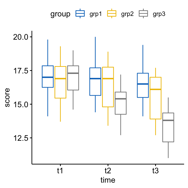
Check assumptions
Outliers
Outliers can be easily identified using box plot methods, implemented in the R function identify_outliers() [rstatix package].
anxiety %>%
  group_by(time, group) %>%
  identify_outliers(score)
## [1] group time id score is.outlier is.extreme
## <0 rows> (or 0-length row.names)There were no extreme outliers.
Note that, in the situation where you have extreme outliers, this can be due to: 1) data entry errors, measurement errors or unusual values.
Yo can include the outlier in the analysis anyway if you do not believe the result will be substantially affected. This can be evaluated by comparing the result of the ANOVA with and without the outlier.
It’s also possible to keep the outliers in the data and perform robust ANOVA test using the WRS2 package.
Normality assumption
The normality assumption can be checked by computing Shapiro-Wilk test for each combinations of factor levels. If the data is normally distributed, the p-value should be greater than 0.05.
anxiety %>%
  group_by(time, group) %>%
  shapiro_test(score)
## # A tibble: 9 x 5
## group time variable statistic p
## <fct> <fct> <chr> <dbl> <dbl>
## 1 grp1 t1 score 0.964 0.769
## 2 grp2 t1 score 0.977 0.949
## 3 grp3 t1 score 0.954 0.588
## 4 grp1 t2 score 0.956 0.624
## 5 grp2 t2 score 0.935 0.328
## 6 grp3 t2 score 0.952 0.558
## # … with 3 more rowsThe score were normally distributed (p > 0.05) for each cell, as assessed by Shapiro-Wilk’s test of normality.
Note that, if your sample size is greater than 50, the normal QQ plot is preferred because at larger sample sizes the Shapiro-Wilk test becomes very sensitive even to a minor deviation from normality.
QQ plot draws the correlation between a given data and the normal distribution.
ggqqplot(anxiety, "score", ggtheme = theme_bw()) +
  facet_grid(time ~ group)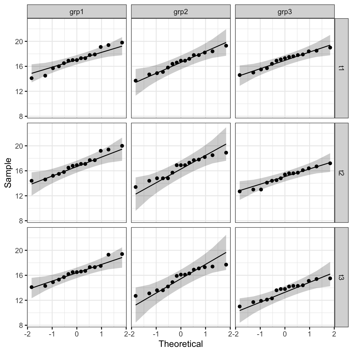
All the points fall approximately along the reference line, for each cell. So we can assume normality of the data.
In the situation where the assumptions are not met, you could consider running the two-way repeated measures ANOVA on the transformed or performing a robust ANOVA test using the WRS2 R package.
Homogneity of variance assumption
The homogeneity of variance assumption of the between-subject factor (group) can be checked using the Levene’s test. The test is performed at each level of time variable:
anxiety %>%
  group_by(time) %>%
  levene_test(score ~ group)
## # A tibble: 3 x 5
## time df1 df2 statistic p
## <fct> <int> <int> <dbl> <dbl>
## 1 t1 2 42 0.176 0.839
## 2 t2 2 42 0.249 0.781
## 3 t3 2 42 0.335 0.717There was homogeneity of variances, as assessed by Levene’s test (p > 0.05).
Note that, if you do not have homogeneity of variances, you can try to transform the outcome (dependent) variable to correct for the unequal variances.
It’s also possible to perform robust ANOVA test using the WRS2 R package.
Homogeneity of covariances assumption
The homogeneity of covariances of the between-subject factor (group) can be evaluated using the Box’s M-test implemented in the rstatix package. If this test is statistically significant (i.e., p < 0.001), you do not have equal covariances, but if the test is not statistically significant (i.e., p > 0.001), you have equal covariances and you have not violated the assumption of homogeneity of covariances.
Note that, the Box’s M is highly sensitive, so unless p < 0.001 and your sample sizes are unequal, ignore it. However, if significant and you have unequal sample sizes, the test is not robust (https://en.wikiversity.org/wiki/Box%27s_M, Tabachnick & Fidell, 2001).
Compute Box’s M-test:
box_m(anxiety[, "score", drop = FALSE], anxiety$group)## # A tibble: 1 x 4
## statistic p.value parameter method
## <dbl> <dbl> <dbl> <chr>
## 1 1.93 0.381 2 Box's M-test for Homogeneity of Covariance MatricesThere was homogeneity of covariances, as assessed by Box’s test of equality of covariance matrices (p > 0.001).
Note that, if you do not have homogeneity of covariances, you could consider separating your analyses into distinct repeated measures ANOVAs for each group. Alternatively, you could omit the interpretation of the interaction term.
Unfortunately, it is difficult to remedy a failure of this assumption. Often, a mixed ANOVA is run anyway and the violation noted.
Assumption of sphericity
As mentioned in previous sections, the assumption of sphericity will be automatically checked during the computation of the ANOVA test using the R function anova_test() [rstatix package]. The Mauchly’s test is internally used to assess the sphericity assumption.
By using the function get_anova_table() [rstatix] to extract the ANOVA table, the Greenhouse-Geisser sphericity correction is automatically applied to factors violating the sphericity assumption.
Computation
# Two-way mixed ANOVA test
res.aov <- anova_test(
  data = anxiety, dv = score, wid = id,
  between = group, within = time
  )
get_anova_table(res.aov)
## ANOVA Table (type II tests)
##
## Effect DFn DFd F p p<.05 ges
## 1 group 2 42 4.35 1.90e-02 * 0.168
## 2 time 2 84 394.91 1.91e-43 * 0.179
## 3 group:time 4 84 110.19 1.38e-32 * 0.108From the output above, it can be seen that, there is a statistically significant two-way interactions between group and time on anxiety score, F(4, 84) = 110.18, p < 0.0001.
Post-hoc tests
A significant two-way interaction indicates that the impact that one factor has on the outcome variable depends on the level of the other factor (and vice versa). So, you can decompose a significant two-way interaction into:
- Simple main effect: run one-way model of the first variable (factor A) at each level of the second variable (factor B),
- Simple pairwise comparisons: if the simple main effect is significant, run multiple pairwise comparisons to determine which groups are different.
For a non-significant two-way interaction, you need to determine whether you have any statistically significant main effects from the ANOVA output.
Procedure for a significant two-way interaction
Simple main effect of group variable. In our example, we’ll investigate the effect of the between-subject factor group on anxiety score at every time point.
# Effect of group at each time point
one.way <- anxiety %>%
  group_by(time) %>%
  anova_test(dv = score, wid = id, between = group) %>%
  get_anova_table() %>%
  adjust_pvalue(method = "bonferroni")
one.way
## # A tibble: 3 x 9
## time Effect DFn DFd F p `p<.05` ges p.adj
## <fct> <chr> <dbl> <dbl> <dbl> <dbl> <chr> <dbl> <dbl>
## 1 t1 group 2 42 0.365 0.696 "" 0.017 1
## 2 t2 group 2 42 5.84 0.006 * 0.218 0.018
## 3 t3 group 2 42 13.8 0.0000248 * 0.396 0.0000744# Pairwise comparisons between group levels
pwc <- anxiety %>%
group_by(time) %>%
pairwise_t_test(score ~ group, p.adjust.method = "bonferroni")
pwc## # A tibble: 9 x 10
## time .y. group1 group2 n1 n2 p p.signif p.adj p.adj.signif
## * <fct> <chr> <chr> <chr> <int> <int> <dbl> <chr> <dbl> <chr>
## 1 t1 score grp1 grp2 15 15 0.43 ns 1 ns
## 2 t1 score grp1 grp3 15 15 0.895 ns 1 ns
## 3 t1 score grp2 grp3 15 15 0.51 ns 1 ns
## 4 t2 score grp1 grp2 15 15 0.435 ns 1 ns
## 5 t2 score grp1 grp3 15 15 0.00212 ** 0.00636 **
## 6 t2 score grp2 grp3 15 15 0.0169 * 0.0507 ns
## # … with 3 more rowsConsidering the Bonferroni adjusted p-value (p.adj), it can be seen that the simple main effect of group was significant at t2 (p = 0.018) and t3 (p < 0.0001) but not at t1 (p = 1).
Pairwise comparisons show that the mean anxiety score was significantly different in grp1 vs grp3 comparison at t2 (p = 0.0063); in grp1 vs grp3 (p < 0.0001) and in grp2 vs grp3 (p = 0.0013) at t3.
Simple main effects of time variable. It’s also possible to perform the same analyze for the within-subject time variable at each level of group as shown in the following R code. You don’t necessarily need to do this analysis.
# Effect of time at each level of exercises group
one.way2 <- anxiety %>%
  group_by(group) %>%
  anova_test(dv = score, wid = id, within = time) %>%
  get_anova_table() %>%
  adjust_pvalue(method = "bonferroni")
one.way2
## # A tibble: 3 x 9
## group Effect DFn DFd F p `p<.05` ges p.adj
## <fct> <chr> <dbl> <dbl> <dbl> <dbl> <chr> <dbl> <dbl>
## 1 grp1 time 2 28 14.8 4.05e- 5 * 0.024 1.21e- 4
## 2 grp2 time 2 28 77.5 3.88e-12 * 0.086 1.16e-11
## 3 grp3 time 2 28 490. 1.64e-22 * 0.531 4.92e-22# Pairwise comparisons between time points at each group levels
# Paired t-test is used because we have repeated measures by time
pwc2 <- anxiety %>%
group_by(group) %>%
pairwise_t_test(
score ~ time, paired = TRUE,
p.adjust.method = "bonferroni"
) %>%
select(-df, -statistic, -p) # Remove details
pwc2## # A tibble: 9 x 8
## group .y. group1 group2 n1 n2 p.adj p.adj.signif
## * <fct> <chr> <chr> <chr> <int> <int> <dbl> <chr>
## 1 grp1 score t1 t2 15 15 0.194 ns
## 2 grp1 score t1 t3 15 15 0.002 **
## 3 grp1 score t2 t3 15 15 0.006 **
## 4 grp2 score t1 t2 15 15 0.268 ns
## 5 grp2 score t1 t3 15 15 0.000000151 ****
## 6 grp2 score t2 t3 15 15 0.0000000612 ****
## # … with 3 more rowsThere was a statistically significant effect of time on anxiety score for each of the three groups. Using pairwise paired t-test comparisons, it can be seen that for grp1 and grp2, the mean anxiety score was not statistically significantly different between t1 and t2 time points.
The pairwise comparisons t1 vs t3 and t2 vs t3 were statistically significantly different for all groups.
Procedure for non-significant two-way interaction
If the interaction is not significant, you need to interpret the main effects for each of the two variables: group and `time. A significant main effect can be followed up with pairwise comparisons.
In our example, there was a statistically significant main effects of group (F(2, 42) = 4.35, p = 0.02) and time (F(2, 84) = 394.91, p < 0.0001) on the anxiety score.
Perform multiple pairwise paired t-tests for the time variable, ignoring group. P-values are adjusted using the Bonferroni multiple testing correction method.
anxiety %>%
  pairwise_t_test(
    score ~ time, paired = TRUE,
    p.adjust.method = "bonferroni"
  )
All pairwise comparisons are significant.
You can perform a similar analysis for the group variable.
anxiety %>%
  pairwise_t_test(
    score ~ group,
    p.adjust.method = "bonferroni"
  )
All pairwise comparisons are significant except grp1 vs grp2.
Report
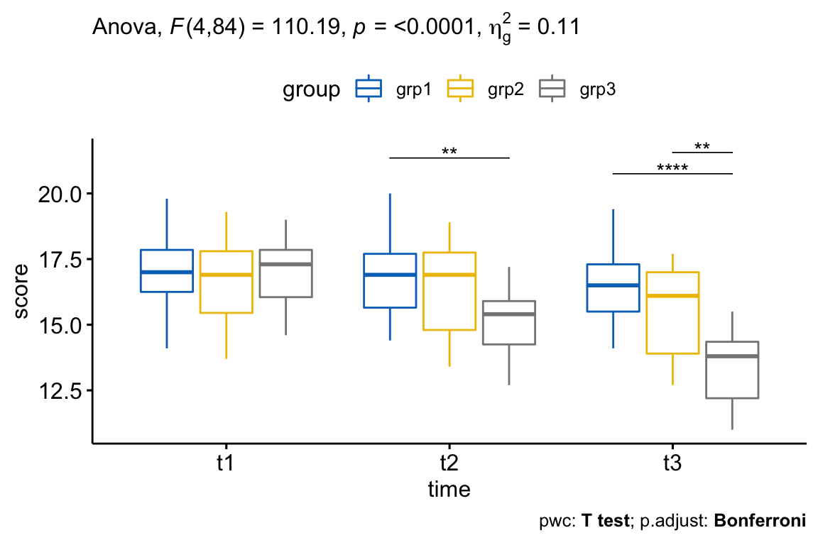
There was a statistically significant interaction between exercises group and time in explaining the anxiety score, F(4, 84) = 110.19, p < 0.0001.
Considering the Bonferroni adjusted p-value, the simple main effect of exercises group was significant at t2 (p = 0.018) and t3 (p < 0.0001) but not at t1 (p = 1).
Pairwise comparisons show that the mean anxiety score was significantly different in grp1 vs grp3 comparison at t2 (p = 0.0063); in grp1 vs grp3 (p < 0.0001) and in grp2 vs grp3 (p = 0.0013) at t3.
Note that, for the plot below, we only need the pairwise comparison results for t2 and t3 but not for t1 (because the simple main effect of exercises group was not significant at this time point). We’ll filter the comparison results accordingly.
# Visualization: boxplots with p-values
pwc <- pwc %>% add_xy_position(x = "time")
pwc.filtered <- pwc %>% filter(time != "t1")
bxp +
  stat_pvalue_manual(pwc.filtered, tip.length = 0, hide.ns = TRUE) +
  labs(
    subtitle = get_test_label(res.aov, detailed = TRUE),
    caption = get_pwc_label(pwc)
  )
Three-way mixed ANOVA: 2 between- and 1 within-subjects factors
This section describes how to compute the three-way mixed ANOVA, in R, for a situation where you have two between-subjects factors and one within-subjects factor.
This setting is for investigating group differences over time (i.e., the within-subjects factor) where groups are formed by the combination of two between-subjects factors. For example, you might want to understand how performance score changes over time (e.g., 0, 4 and 8 months) depending on gender (i.e., male/female) and stress (low, moderate and high stress).
Data preparation
We’ll use performance dataset [datarium package] containing the performance score measures of participants at two time points. The aim of this study is to evaluate the effect of gender and stress on performance score.
The data contains the following variables:
- Performance score (outcome or dependent variable) measured at two time points,
t1andt2. - Two between-subjects factors:
gender(levels: male and female) andstress(low, moderate, high)
- One within-subjects factor,
time, which has two time points:t1andt2.
Load and inspect the data by showing one random row by group:
# Load and inspect the data
# Wide format
set.seed(123)
data("performance", package = "datarium")
performance %>% sample_n_by(gender, stress, size = 1)
## # A tibble: 6 x 5
## id gender stress t1 t2
## <int> <fct> <fct> <dbl> <dbl>
## 1 3 male low 5.63 5.47
## 2 18 male moderate 5.57 5.78
## 3 25 male high 5.48 5.74
## 4 39 female low 5.50 5.66
## 5 50 female moderate 5.96 5.32
## 6 51 female high 5.59 5.06# Gather the columns t1, t2 and t3 into long format.
# Convert id and time into factor variables
performance <- performance %>%
gather(key = "time", value = "score", t1, t2) %>%
convert_as_factor(id, time)
# Inspect some random rows of the data by groups
set.seed(123)
performance %>% sample_n_by(gender, stress, time, size = 1)## # A tibble: 12 x 5
## id gender stress time score
## <fct> <fct> <fct> <fct> <dbl>
## 1 3 male low t1 5.63
## 2 8 male low t2 5.92
## 3 15 male moderate t1 5.96
## 4 19 male moderate t2 5.76
## 5 30 male high t1 5.38
## 6 21 male high t2 5.64
## # … with 6 more rowsSummary statistics
Group the data by gender, stress and time, and then compute some summary statistics of the score variable: mean and sd (standard deviation)
performance %>%
  group_by(gender, stress, time ) %>%
  get_summary_stats(score, type = "mean_sd")
## # A tibble: 12 x 7
## gender stress time variable n mean sd
## <fct> <fct> <fct> <chr> <dbl> <dbl> <dbl>
## 1 male low t1 score 10 5.72 0.19
## 2 male low t2 score 10 5.70 0.143
## 3 male moderate t1 score 10 5.72 0.193
## 4 male moderate t2 score 10 5.77 0.155
## 5 male high t1 score 10 5.48 0.121
## 6 male high t2 score 10 5.64 0.195
## # … with 6 more rowsVisualization
Create box plots of performance score by gender colored by stress levels and faceted by time:
bxp <- ggboxplot(
  performance, x = "gender", y = "score",
  color = "stress", palette = "jco",
  facet.by =  "time"
  )
bxp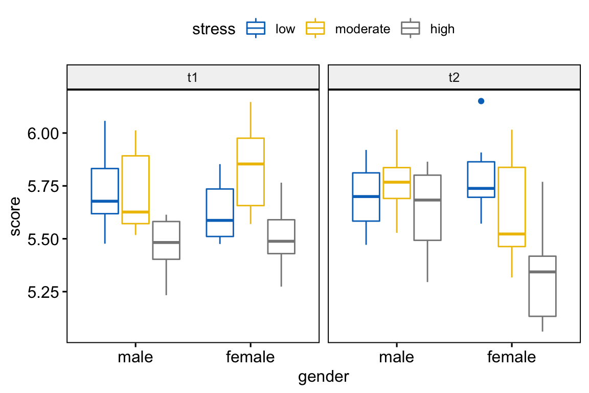
Check assumptions
Outliers
performance %>%
  group_by(gender, stress, time) %>%
  identify_outliers(score)
## # A tibble: 1 x 7
## gender stress time id score is.outlier is.extreme
## <fct> <fct> <fct> <fct> <dbl> <lgl> <lgl>
## 1 female low t2 36 6.15 TRUE FALSEThere were no extreme outliers.
Normality assumption
Compute Shapiro-Wilk test for each combinations of factor levels:
performance %>%
  group_by(gender, stress, time ) %>%
  shapiro_test(score)
## # A tibble: 12 x 6
## gender stress time variable statistic p
## <fct> <fct> <fct> <chr> <dbl> <dbl>
## 1 male low t1 score 0.942 0.574
## 2 male low t2 score 0.966 0.849
## 3 male moderate t1 score 0.848 0.0547
## 4 male moderate t2 score 0.958 0.761
## 5 male high t1 score 0.915 0.319
## 6 male high t2 score 0.925 0.403
## # … with 6 more rowsThe score were normally distributed (p > 0.05) for each cell, as assessed by Shapiro-Wilk’s test of normality.
Create QQ plot for each cell of design:
ggqqplot(performance, "score", ggtheme = theme_bw()) +
  facet_grid(time ~ stress, labeller = "label_both")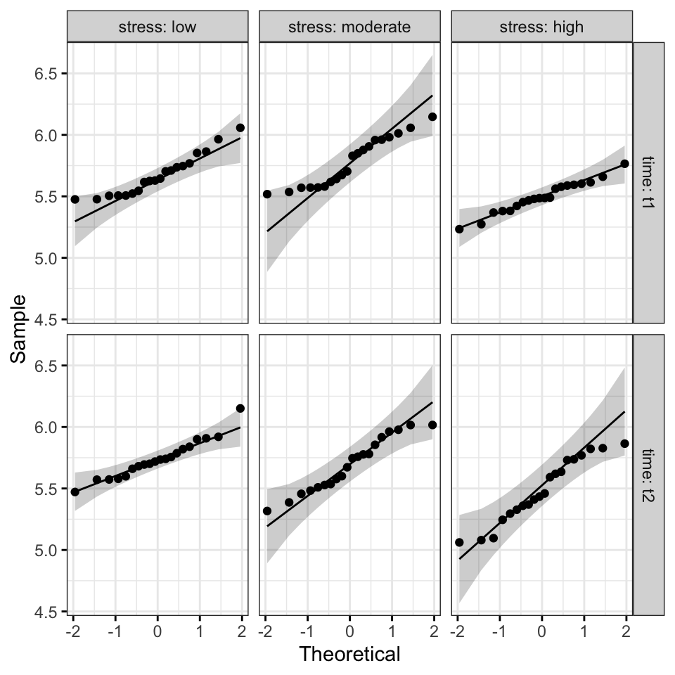
All the points fall approximately along the reference line, for each cell. So we can assume normality of the data.
Homogneity of variance assumption
Compute the Levene’s test at each level of the within-subjects factor, here time variable:
performance %>%
  group_by(time) %>%
  levene_test(score ~ gender*stress)
## # A tibble: 2 x 5
## time df1 df2 statistic p
## <fct> <int> <int> <dbl> <dbl>
## 1 t1 5 54 0.974 0.442
## 2 t2 5 54 0.722 0.610There was homogeneity of variances, as assessed by Levene’s test of homogeneity of variance (p > .05).
Assumption of sphericity
As mentioned in the two-way mixed ANOVA section, the Mauchly’s test of sphericity and the sphericity corrections are internally done using the R function anova_test() and get_anova_table() [rstatix package].
Computation
res.aov <- anova_test(
  data = performance, dv = score, wid = id,
  within = time, between = c(gender, stress)
  )
get_anova_table(res.aov)
## ANOVA Table (type II tests)
##
## Effect DFn DFd F p p<.05 ges
## 1 gender 1 54 2.406 1.27e-01 0.023000
## 2 stress 2 54 21.166 1.63e-07 * 0.288000
## 3 time 1 54 0.063 8.03e-01 0.000564
## 4 gender:stress 2 54 1.554 2.21e-01 0.029000
## 5 gender:time 1 54 4.730 3.40e-02 * 0.041000
## 6 stress:time 2 54 1.821 1.72e-01 0.032000
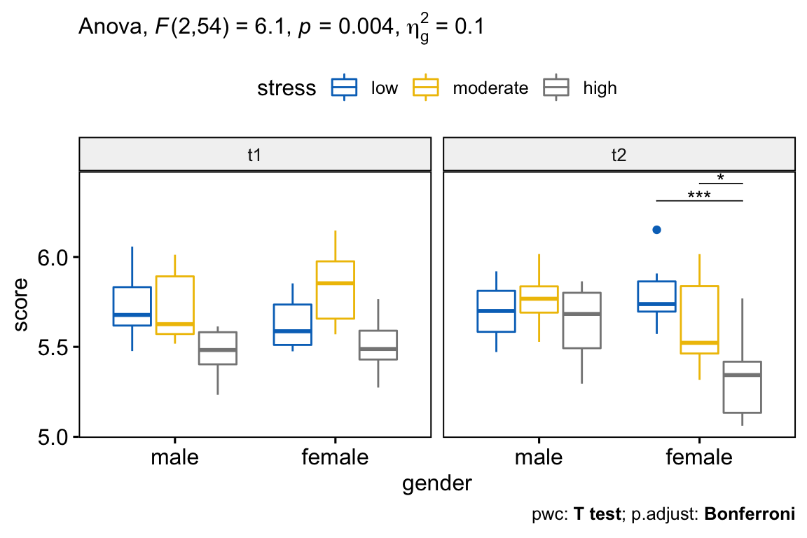
## 7 gender:stress:time 2 54 6.101 4.00e-03 * 0.098000There was a statistically significant three-way interaction between time, gender, and stress F(2, 54) = 6.10, p = 0.004.
Post-hoc tests
If there is a significant three-way interaction effect, you can decompose it into:
- Simple two-way interaction: run two-way interaction at each level of third variable,
- Simple simple main effect: run one-way model at each level of second variable, and
- simple simple pairwise comparisons: run pairwise or other post-hoc comparisons if necessary.
If you do not have a statistically significant three-way interaction, you need to determine whether you have any statistically significant two-way interaction from the ANOVA output. A significant two-way interaction can be followed up by a simple main effect analysis, which can be followed up by simple pairwise comparisons if significant.
In this section we’ll describe the procedure for a significant three-way interaction.
Compute simple two-way interaction
You are free to decide which two variables will form the simple two-way interactions and which variable will act as the third variable.
In the following R code, we have considered the simple two-way interaction of gender*stress at each level of time.
Group the data by time (the within-subject factors) and analyze the simple two-way interaction between gender and stress, which are the between-subjects factors.
# two-way interaction at each time levels
two.way <- performance %>%
  group_by(time) %>%
  anova_test(dv = score, wid = id, between = c(gender, stress))
two.way
## # A tibble: 6 x 8
## time Effect DFn DFd F p `p<.05` ges
## <fct> <chr> <dbl> <dbl> <dbl> <dbl> <chr> <dbl>
## 1 t1 gender 1 54 0.186 0.668 "" 0.003
## 2 t1 stress 2 54 14.9 0.00000723 * 0.355
## 3 t1 gender:stress 2 54 2.12 0.131 "" 0.073
## 4 t2 gender 1 54 5.97 0.018 * 0.1
## 5 t2 stress 2 54 9.60 0.000271 * 0.262
## 6 t2 gender:stress 2 54 4.95 0.011 * 0.155There was a statistically significant simple two-way interaction of gender and stress at t2, F(2, 54) = 4.95, p = 0.011, but not at t1, F(2, 54) = 2.12, p = 0.13.
Note that, statistical significance of a simple two-way interaction was accepted at a Bonferroni-adjusted alpha level of 0.025. This corresponds to the current level you declare statistical significance at (i.e., p < 0.05) divided by the number of simple two-way interaction you are computing (i.e., 2).
Compute simple simple main effects
A statistically significant simple two-way interaction can be followed up with simple simple main effects.
In our example, you could therefore investigate the effect of stress on the performance score at every level of gender or investigate the effect of gender at every level of stress.
Note that, you will only need to do this for the simple two-way interaction for “t2” as this was the only simple two-way interaction that was statistically significant.
Group the data by time and gender, and analyze the simple main effect of stress on performance score:
stress.effect <- performance %>%
  group_by(time, gender) %>%
  anova_test(dv = score, wid = id, between = stress)
stress.effect %>% filter(time == "t2")
## # A tibble: 2 x 9
## gender time Effect DFn DFd F p `p<.05` ges
## <fct> <fct> <chr> <dbl> <dbl> <dbl> <dbl> <chr> <dbl>
## 1 male t2 stress 2 27 1.57 0.227 "" 0.104
## 2 female t2 stress 2 27 10.5 0.000416 * 0.438In the table above, we only need the results for time = t2. Statistical significance of a simple simple main effect was accepted at a Bonferroni-adjusted alpha level of 0.025, that is 0.05 divided y the number of simple simple main effects you are computing (i.e., 2).
There was a statistically significant simple simple main effect of stress on the performance score for female at t2 time point, F(2, 27) = 10.5, p = 0.0004, but not for males, F(2, 27) = 1.57, p = 0.23.
Compute simple simple comparisons
A statistically significant simple simple main effect can be followed up by multiple pairwise comparisons to determine which group means are different.
Note that, you will only need to concentrate on the pairwise comparison results for female, because the effect of stress was significant for female only in the previous section.
Group the data by time and gender, and perform pairwise comparisons between stress levels with Bonferroni adjustment:
# Fit pairwise comparisons
pwc <- performance %>%
  group_by(time, gender) %>%
  pairwise_t_test(score ~ stress, p.adjust.method = "bonferroni") %>%
  select(-p, -p.signif) # Remove details
# Focus on the results of "female" at t2
pwc %>% filter(time == "t2", gender == "female")
## # A tibble: 3 x 9
## gender time .y. group1 group2 n1 n2 p.adj p.adj.signif
## <fct> <fct> <chr> <chr> <chr> <int> <int> <dbl> <chr>
## 1 female t2 score low moderate 10 10 0.323 ns
## 2 female t2 score low high 10 10 0.000318 ***
## 3 female t2 score moderate high 10 10 0.0235 *For female, the mean performance score was statistically significantly different between low and high stress levels (p < 0.001) and between moderate and high stress levels (p = 0.023).
There was no significant difference between low and moderate stress groups (p = 0.32)
Report
A three-way mixed ANOVA was performed to evaluate the effects of gender, stress and time on performance score.
There were no extreme outliers, as assessed by box plot method. The data was normally distributed, as assessed by Shapiro-Wilk’s test of normality (p > 0.05). There was homogeneity of variances (p > 0.05) as assessed by Levene’s test of homogeneity of variances.
There was a statistically significant three-way interaction between gender, stress and time, F(2, 54) = 6.10, p = 0.004.
For the simple two-way interactions and simple simple main effects, a Bonferroni adjustment was applied leading to statistical significance being accepted at the p < 0.025 level.
There was a statistically significant simple two-way interaction between gender and stress at time point t2, F(2, 54) = 4.95, p = 0.011, but not at t1, F(2, 54) = 2.12, p = 0.13.
There was a statistically significant simple simple main effect of stress on the performance score for female at t2 time point, F(2, 27) = 10.5, p = 0.0004, but not for males, F(2, 27) = 1.57, p = 0.23.
All simple simple pairwise comparisons were run between the different stress groups for female at time point t2. A Bonferroni adjustment was applied.
The mean performance score was statistically significantly different between low and high stress levels (p < 0.001) and between moderate and high stress levels (p = 0.024). There was no significant difference between low and moderate stress groups (p = 0.32).
# Visualization: box plots with p-values
pwc <- pwc %>% add_xy_position(x = "gender")
pwc.filtered <- pwc %>% filter(time == "t2", gender == "female")
bxp +
  stat_pvalue_manual(pwc.filtered, tip.length = 0, hide.ns = TRUE) +
  labs(
    subtitle = get_test_label(res.aov, detailed = TRUE),
    caption = get_pwc_label(pwc)
  )
Three-way Mixed ANOVA: 1 between- and 2 within-subjects factors
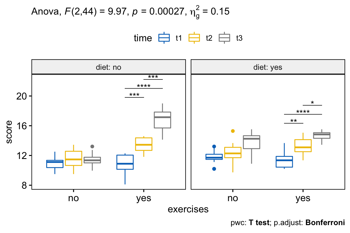
This section describes how to compute the three-way mixed ANOVA, in R, for a situation where you have one between-subjects factor and two within-subjects factors. For example, you might want to understand how weight loss score differs in individuals doing exercises vs not doing exercises over three time points (t1, t2, t3) depending on participant diets (diet:no and diet:yes).
Data preparation
We’ll use the weightloss dataset available in the datarium package. This dataset was originally created for three-way repeated measures ANOVA. However, for our example in this article, we’ll modify slightly the data so that it corresponds to a three-way mixed design.
A researcher wanted to assess the effect of time on weight loss score depending on exercises programs and diet.
The weight loss score was measured in two different groups: a group of participants doing exercises (exercises:yes) and in another group not doing exercises (excises:no).
Each participant was also enrolled in two trials: (1) no diet and (2) diet. The order of the trials was counterbalanced and sufficient time was allowed between trials to allow any effects of previous trials to have dissipated.
Each trial lasted 9 weeks and the weight loss score was measured at the beginning of each trial (t1), at the midpoint of each trial (t2) and at the end of each trial (t3).
In this study design, 24 individuals were recruited. Of these 24 participants, 12 belongs to the exercises:no group and 12 were in exercises:yes group. The 24 participants were enrolled in two successive trials (diet:no and diet:yes) and the weight loss score was repeatedly measured at three time points.
In this setting, we have:
- one dependent (or outcome) variable:
score - One between-subjects factor:
exercises - two within-subjects factors:
dietendtime
Three-way mixed ANOVA can be performed in order to determine whether there is a significant interaction between diet, exercises and time on the weight loss score.
Load the data and inspect some random rows by group:
# Load the original data
# Wide format
data("weightloss", package = "datarium")
# Modify it to have three-way mixed design
weightloss <- weightloss %>%
  mutate(id = rep(1:24, 2)) # two trials
# Show one random row by group
set.seed(123)
weightloss %>% sample_n_by(diet, exercises, size = 1)
## # A tibble: 4 x 6
## id diet exercises t1 t2 t3
## <int> <fct> <fct> <dbl> <dbl> <dbl>
## 1 4 no no 11.1 9.5 11.1
## 2 22 no yes 10.2 11.8 17.4
## 3 5 yes no 11.6 13.4 13.9
## 4 23 yes yes 12.7 12.7 15.1# Gather the columns t1, t2 and t3 into long format.
# Convert id and time into factor variables
weightloss <- weightloss %>%
gather(key = "time", value = "score", t1, t2, t3) %>%
convert_as_factor(id, time)
# Inspect some random rows of the data by groups
set.seed(123)
weightloss %>% sample_n_by(diet, exercises, time, size = 1)## # A tibble: 12 x 5
## id diet exercises time score
## <fct> <fct> <fct> <fct> <dbl>
## 1 4 no no t1 11.1
## 2 10 no no t2 10.7
## 3 5 no no t3 12.3
## 4 23 no yes t1 10.2
## 5 24 no yes t2 13.2
## 6 13 no yes t3 15.8
## # … with 6 more rowsSummary statistics
Group the data by exercises, diet and time, and then compute some summary statistics of the score variable: mean and sd (standard deviation)
weightloss %>%
  group_by(exercises, diet, time) %>%
  get_summary_stats(score, type = "mean_sd")
## # A tibble: 12 x 7
## diet exercises time variable n mean sd
## <fct> <fct> <fct> <chr> <dbl> <dbl> <dbl>
## 1 no no t1 score 12 10.9 0.868
## 2 no no t2 score 12 11.6 1.30
## 3 no no t3 score 12 11.4 0.935
## 4 yes no t1 score 12 11.7 0.938
## 5 yes no t2 score 12 12.4 1.42
## 6 yes no t3 score 12 13.8 1.43
## # … with 6 more rowsVisualization
Create box plots of weightloss score by exercises groups, colored by time points and faceted by diet trials:
bxp <- ggboxplot(
  weightloss, x = "exercises", y = "score",
  color = "time", palette = "jco",
  facet.by = "diet", short.panel.labs = FALSE
  )
bxp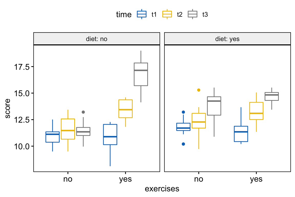
Check assumptions
Outliers
weightloss %>%
  group_by(diet, exercises, time) %>%
  identify_outliers(score)
## # A tibble: 5 x 7
## diet exercises time id score is.outlier is.extreme
## <fct> <fct> <fct> <fct> <dbl> <lgl> <lgl>
## 1 no no t3 2 13.2 TRUE FALSE
## 2 yes no t1 1 10.2 TRUE FALSE
## 3 yes no t1 3 13.2 TRUE FALSE
## 4 yes no t1 4 10.2 TRUE FALSE
## 5 yes no t2 10 15.3 TRUE FALSEThere were no extreme outliers.
Normality assumption
Compute Shapiro-Wilk test for each combinations of factor levels:
weightloss %>%
  group_by(diet, exercises, time) %>%
  shapiro_test(score)
## # A tibble: 12 x 6
## diet exercises time variable statistic p
## <fct> <fct> <fct> <chr> <dbl> <dbl>
## 1 no no t1 score 0.917 0.264
## 2 no no t2 score 0.957 0.743
## 3 no no t3 score 0.965 0.851
## 4 no yes t1 score 0.922 0.306
## 5 no yes t2 score 0.912 0.229
## 6 no yes t3 score 0.953 0.674
## # … with 6 more rowsThe weight loss score was normally distributed (p > 0.05), as assessed by Shapiro-Wilk’s test of normality.
Create QQ plot for each cell of design:
ggqqplot(weightloss, "score", ggtheme = theme_bw()) +
  facet_grid(diet + exercises ~ time, labeller = "label_both")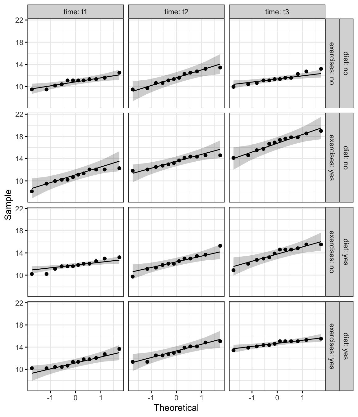
From the plot above, as all the points fall approximately along this reference line, we can assume normality.
Homogneity of variance assumption
Compute the Levene’s test after grouping the data by diet and time categories:
weightloss %>%
  group_by(diet, time) %>%
  levene_test(score ~ exercises)
## # A tibble: 6 x 6
## diet time df1 df2 statistic p
## <fct> <fct> <int> <int> <dbl> <dbl>
## 1 no t1 1 22 2.44 0.132
## 2 no t2 1 22 0.691 0.415
## 3 no t3 1 22 2.87 0.105
## 4 yes t1 1 22 0.376 0.546
## 5 yes t2 1 22 0.0574 0.813
## 6 yes t3 1 22 5.14 0.0336There was homogeneity of variances for all cells (p > 0.05), except for the condition diet:yes at time:t3 (p = 0.034), as assessed by Levene’s test of homogeneity of variance.
Note that, if you do not have homogeneity of variances, you can try to transform the outcome (dependent) variable to correct for the unequal variances.
If group sample sizes are (approximately) equal, run the three-way mixed ANOVA anyway because it is somewhat robust to heterogeneity of variance in these circumstances.
It’s also possible to perform robust ANOVA test using the WRS2 R package.
Assumption of sphericity
As mentioned in the two-way mixed ANOVA section, the Mauchly’s test of sphericity and the sphericity corrections are internally done using the R function anova_test() and get_anova_table() [rstatix package].
Computation
res.aov <- anova_test(
  data = weightloss, dv = score, wid = id,
  between = exercises, within = c(diet, time)
  )
get_anova_table(res.aov)
## ANOVA Table (type II tests)
##
## Effect DFn DFd F p p<.05 ges
## 1 exercises 1 22 38.771 2.88e-06 * 0.284
## 2 diet 1 22 7.912 1.00e-02 * 0.028
## 3 time 2 44 82.199 1.38e-15 * 0.541
## 4 exercises:diet 1 22 51.698 3.31e-07 * 0.157
## 5 exercises:time 2 44 26.222 3.18e-08 * 0.274
## 6 diet:time 2 44 0.784 4.63e-01 0.013
## 7 exercises:diet:time 2 44 9.966 2.69e-04 * 0.147From the output above, it can be seen that there is a statistically significant three-way interactions between exercises, diet and time F(2, 44) = 9.96, p = 0.00027.
Note that, if the three-way interaction is not statistically significant, you need to consult the two-way interactions in the output.
In our example, there was a statistically significant two-way exercises*diet interaction (p < 0.0001), and two-way exercises*time (p < 0.0001). The two-way diet*time interaction was not statistically significant (p = 0.46).
Post-hoc tests
If there is a significant three-way interaction effect, you can decompose it into:
- Simple two-way interaction: run two-way interaction at each level of third variable,
- Simple simple main effect: run one-way model at each level of second variable, and
- simple simple pairwise comparisons: run pairwise or other post-hoc comparisons if necessary.
If you do not have a statistically significant three-way interaction, you need to determine whether you have any statistically significant two-way interaction from the ANOVA output. You can follow up a significant two-way interaction by simple main effects analyses and pairwise comparisons between groups if necessary.
In this section we’ll describe the procedure for a significant three-way interaction.
Compute simple two-way interaction
In this example, we’ll consider the diet*time interaction at each level of exercises. Group the data by exercises and analyze the simple two-way interaction between diet and time:
# Two-way ANOVA at each exercises group level
two.way <- weightloss %>%
  group_by(exercises) %>%
  anova_test(dv = score, wid = id, within = c(diet, time))
two.way
## # A tibble: 2 x 2
## exercises anova
## <fct> <list>
## 1 no <anov_tst>
## 2 yes <anov_tst># Extract anova table
get_anova_table(two.way)## # A tibble: 6 x 8
## exercises Effect DFn DFd F p `p<.05` ges
## <fct> <chr> <dbl> <dbl> <dbl> <dbl> <chr> <dbl>
## 1 no diet 1 11 56.4 1.18e- 5 * 0.262
## 2 no time 2 22 5.90 9.00e- 3 * 0.181
## 3 no diet:time 2 22 2.91 7.60e- 2 "" 0.09
## 4 yes diet 1 11 8.60 1.40e- 2 * 0.066
## 5 yes time 2 22 148. 1.73e-13 * 0.746
## 6 yes diet:time 2 22 7.81 3.00e- 3 * 0.216There was a statistically significant simple two-way interaction between diet and time for exercises:yes group, F(2, 22) = 7.81, p = 0.0027, but not for exercises:no group, F(2, 22) = 2.91, p = 0.075.
Note that, statistical significance of a simple two-way interaction was accepted at a Bonferroni-adjusted alpha level of 0.025. This corresponds to the current level you declare statistical significance at (i.e., p < 0.05) divided by the number of simple two-way interaction you are computing (i.e., 2).
Compute simple simple main effect
A statistically significant simple two-way interaction can be followed up with simple simple main effects.
In our example, you could therefore investigate the effect of time on the weight loss score at every level of diet and/or investigate the effect of diet at every level of time.
Note that, you will only need to do this for the simple two-way interaction for “exercises:yes” group, as this was the only simple two-way interaction that was statistically significant.
Group the data by exercises and diet, and analyze the simple main effect of time:
time.effect <- weightloss %>%
  group_by(exercises, diet) %>%
  anova_test(dv = score, wid = id, within = time) %>%
  get_anova_table()
time.effect %>% filter(exercises == "yes")
## # A tibble: 2 x 9
## diet exercises Effect DFn DFd F p `p<.05` ges
## <fct> <fct> <chr> <dbl> <dbl> <dbl> <dbl> <chr> <dbl>
## 1 no yes time 2 22 78.8 9.30e-11 * 0.801
## 2 yes yes time 2 22 30.9 4.06e- 7 * 0.655In the table above, we only need the results for exercises = yes. Statistical significance of a simple simple main effect was accepted at a Bonferroni-adjusted alpha level of 0.025, that is 0.05 divided y the number of simple simple main effects you are computing (i.e., 2).
The simple simple main effect of time on weight loss score was statistically significant under exercises condition for both diet:no (F(2,22) = 78.81, p < 0.0001) and diet:yes (F(2, 22) = 30.92, p < 0.0001) groups.
Compute simple simple comparisons
A statistically significant simple simple main effect can be followed up by multiple pairwise comparisons to determine which group means are different.
Recall that, you will only need to concentrate on the pairwise comparison results for exercises:yes.
Group the data by exercises and diet, and perform pairwise comparisons between time points with Bonferroni adjustment. Paired t-test is used:
# compute pairwise comparisons
pwc <- weightloss %>%
  group_by(exercises, diet) %>%
  pairwise_t_test(
    score ~ time, paired = TRUE,
    p.adjust.method = "bonferroni"
    ) %>%
  select(-statistic, -df) # Remove details
# Focus on the results of exercises:yes group
pwc %>% filter(exercises == "yes") %>%
  select(-p)    # Remove p column
## # A tibble: 6 x 9
## diet exercises .y. group1 group2 n1 n2 p.adj p.adj.signif
## <fct> <fct> <chr> <chr> <chr> <int> <int> <dbl> <chr>
## 1 no yes score t1 t2 12 12 0.000741 ***
## 2 no yes score t1 t3 12 12 0.0000000121 ****
## 3 no yes score t2 t3 12 12 0.000257 ***
## 4 yes yes score t1 t2 12 12 0.01 **
## 5 yes yes score t1 t3 12 12 0.00000124 ****
## 6 yes yes score t2 t3 12 12 0.02 *All simple simple pairwise comparisons were run between the different time points under exercises condition (i.e., exercises:yes) for diet:no and diet:yes trials. A Bonferroni adjustment was applied.
The mean weight loss score was significantly different in all time point comparisons when exercises are performed (p < 0.05).
Report
A three-way mixed ANOVA was performed to evaluate the effects of diet, exercises and time on weight loss.
There were no extreme outliers, as assessed by box plot method. The data was normally distributed, as assessed by Shapiro-Wilk’s test of normality (p > 0.05). There was homogeneity of variances (p > 0.05) as assessed by Levene’s test of homogeneity of variances. For the three-way interaction effect, Mauchly’s test of sphericity indicated that the assumption of sphericity was met (p > 0.05).
There was a statistically significant three-way interaction between exercises, diet and time F(2, 44) = 9.96, p < 0.001.
For the simple two-way interactions and simple simple main effects, a Bonferroni adjustment was applied leading to statistical significance being accepted at the p < 0.025 level.
There was a statistically significant simple two-way interaction between diet and time for exercises:yes group, F(2, 22) = 7.81, p = 0.0027, but not for exercises:no group, F(2, 22) = 2.91, p = 0.075.
The simple simple main effect of time on weight loss score was statistically significant under exercises condition for both diet:no (F(2,22) = 78.81, p < 0.0001) and diet:yes (F(2, 22) = 30.92, p < 0.0001) groups.
All simple simple pairwise comparisons were run between the different time points under exercises condition (i.e., exercises:yes) for diet:no and diet:yes trials. A Bonferroni adjustment was applied. The mean weight loss score was significantly different in all time point comparisons when exercises are performed (p < 0.05).
# Visualization: box plots with p-values
pwc <- pwc %>% add_xy_position(x = "exercises")
pwc.filtered <- pwc %>% filter(exercises == "yes")
bxp +
  stat_pvalue_manual(pwc.filtered, tip.length = 0, hide.ns = TRUE) +
  labs(
    subtitle = get_test_label(res.aov, detailed = TRUE),
    caption = get_pwc_label(pwc)
  )
Summary
This article describes how to compute and interpret mixed ANOVA in R. We also explain the assumptions made by mixed ANOVA tests and provide practical examples of R codes to check whether the test assumptions are met.
Recommended for you
This section contains best data science and self-development resources to help you on your path.
Books - Data Science
Our Books
- Practical Guide to Cluster Analysis in R by A. Kassambara (Datanovia)
- Practical Guide To Principal Component Methods in R by A. Kassambara (Datanovia)
- Machine Learning Essentials: Practical Guide in R by A. Kassambara (Datanovia)
- R Graphics Essentials for Great Data Visualization by A. Kassambara (Datanovia)
- GGPlot2 Essentials for Great Data Visualization in R by A. Kassambara (Datanovia)
- Network Analysis and Visualization in R by A. Kassambara (Datanovia)
- Practical Statistics in R for Comparing Groups: Numerical Variables by A. Kassambara (Datanovia)
- Inter-Rater Reliability Essentials: Practical Guide in R by A. Kassambara (Datanovia)
Others
- R for Data Science: Import, Tidy, Transform, Visualize, and Model Data by Hadley Wickham & Garrett Grolemund
- Hands-On Machine Learning with Scikit-Learn, Keras, and TensorFlow: Concepts, Tools, and Techniques to Build Intelligent Systems by Aurelien Géron
- Practical Statistics for Data Scientists: 50 Essential Concepts by Peter Bruce & Andrew Bruce
- Hands-On Programming with R: Write Your Own Functions And Simulations by Garrett Grolemund & Hadley Wickham
- An Introduction to Statistical Learning: with Applications in R by Gareth James et al.
- Deep Learning with R by François Chollet & J.J. Allaire
- Deep Learning with Python by François Chollet
Version:
 Français

Thanks so much for all the great info, your site has been extremely helpful. I’m having a hard time successfully running rstatix::anova_test to check the assumption of sphericity in my dataset; I continue running into the error below. The within and between subjects factors have 3 and 2 levels, respectively, so I’m not sure why I get this error. I wonder if it has something to do with the block factor (the experiment was in a randomized complete block design), which I can’t figure out how to fit into the command. Can you offer any guidance?
# rstatix::anova_test
mauch.x15 Warning: NA detected in rows: 8.
#> Removing this rows before the analysis.
#> Error in `contrasts<-`(`*tmp*`, value = contr.funs[1 + isOF[nn]]): contrasts can be applied only to factors with 2 or more levels
Please provide the rstatix command you used so that I can reproduce the error, thanks
mauch.x15 <- anova_test(data = df,
dv = x,
wid = new.id,
between = sub,
within = time)
Just wanted to chime in to say I am having a similar error.
res.aov <- anova_test(
data = DATA, dv = logQ, wid = momTC2,
between = treatment, within = type
)
logQ: continuous response variable
momTC2: individual ID , each one appearing twice
treatment: two levels
type: repeated factor with two time points
Overall, your site is incredibly clear and helpful. Just not sure how to work through this error.
Thanks!
Thank you, you need to keep only complete cases in your data as shown below:
I am running in the same error but in my case, there are no missing values. Ps: sorry to post it like this, but I am having issues to use pubr, probably because I am new to R. Still, it is possible to see the data in this example.
> #Loading packages to run analyses
> library(tidyverse)
> library(rstatix)
> library(dplyr)
> library(tidyr)
>
> ###Loading data
>
> textFile data
> data
rowId SubjectID Group trialName stimName StimType Measure
1 1 1 group1 trial3 stimA A 0.55908866
2 2 2 group1 trial3 stimA A 0.98884446
3 3 3 group2 trial3 stimA A 0.00000000
4 4 4 group2 trial3 stimA A 0.27067991
5 5 5 group3 trial3 stimA A 0.37169285
6 6 6 group3 trial3 stimA A 0.42113984
7 7 1 group1 trial3 stimB B 0.00000000
8 8 2 group1 trial3 stimB B 0.49892807
9 9 3 group2 trial3 stimB B 0.14602589
10 10 4 group2 trial3 stimB B 0.50946555
11 11 5 group3 trial3 stimB B 0.25572820
12 12 6 group3 trial3 stimB B 0.22932966
13 13 1 group1 trial1 stimA A 0.42207604
14 14 2 group1 trial1 stimA A 0.85599588
15 15 3 group2 trial1 stimA A 0.36428381
16 16 4 group2 trial1 stimA A 0.46679336
17 17 5 group3 trial1 stimA A 0.69379734
18 18 6 group3 trial1 stimA A 0.55607716
19 19 1 group1 trial1 stimB B 0.24261465
20 20 2 group1 trial1 stimB B 0.35176384
21 21 3 group2 trial1 stimB B 0.21116215
22 22 4 group2 trial1 stimB B 0.33112544
23 23 5 group3 trial1 stimB B 0.00000000
24 24 6 group3 trial1 stimB B 0.00000000
25 25 1 group1 trial2 stimA A 0.05506943
26 26 2 group1 trial2 stimA A 0.22537470
27 27 3 group2 trial2 stimA A 0.00000000
28 28 4 group2 trial2 stimA A 0.18511144
29 29 5 group3 trial2 stimA A 0.15586156
30 30 6 group3 trial2 stimA A 0.04467100
31 31 1 group1 trial2 stimB B 0.03890585
32 32 2 group1 trial2 stimB B 0.29787709
33 33 3 group2 trial2 stimB B 0.00000000
34 34 4 group2 trial2 stimB B 0.28971992
35 35 5 group3 trial2 stimB B 0.12993238
36 36 6 group3 trial2 stimB B 0.05066011
>
> data % convert_as_factor(SubjectID, Group, trialName, stimName)
>
> str(my_data)
‘data.frame’: 36 obs. of 6 variables:
$ SubjectID: Factor w/ 6 levels “1”,”2″,”3″,”4″,..: 1 2 3 4 5 6 1 2 3 4 …
$ Group : Factor w/ 3 levels “group1″,”group2”,..: 1 1 2 2 3 3 1 1 2 2 …
$ trialName: Factor w/ 3 levels “trial1″,”trial2”,..: 3 3 3 3 3 3 3 3 3 3 …
$ stimName : Factor w/ 2 levels “stimA”,”stimB”: 1 1 1 1 1 1 2 2 2 2 …
$ StimType : chr “A” “A” “A” “A” …
$ Measure : num 0.559 0.989 0 0.271 0.372 …
>
>
> #Trying mixed ANOVA with rstatix
>
> mixed.anova <- anova_test(
+ data = data, dv = Measure, wid = SubjectID,
+ between = Group, within = c(trialName,stimName)
+ )
Error in `contrasts<-`(`*tmp*`, value = contr.funs[1 + isOF[nn]]) :
contrasts can be applied only to factors with 2 or more levels
This worked! Thanks so much, excellent site and help.
Hi Dr. Kassambara,
I found the rstatix package extremely useful for some analyses I have to run on my data. However, I have not been able to run three way ANOVAS. I am not sure what is happening but here is a look at my data.
> str(data_n19_final)
'data.frame':	342 obs. of  16 variables:
 $ SubjectID  : Factor w/ 84 levels "CC10_B_LRC","CC11_A_LFF",..: 6 7 11 13 14 15 17 19 20 21 ...
 $ DateDay1   : chr  "24/03/17" "03/04/17" "18/04/17" "18/04/17" ...
 $ Sex        : chr  "M" "M" "F" "M" ...
 $ DateofBirth: chr  "17/05/86" "26/11/85" "09/04/97" "23/11/90" ...
 $ Age        : int  30 31 20 26 19 21 20 19 20 27 ...
 $ YearsEduc  : int  NA 17 13 16 12 11 15 13 14 18 ...
 $ IDATEE     : int  50 26 47 42 40 44 28 42 41 44 ...
 $ IDATET     : int  45 21 39 NA 56 42 32 37 49 44 ...
 $ Beck       : int  11 1 6 4 19 13 7 10 15 18 ...
 $ CSOrder    : chr  "A5" "B5" "A3" "A4" ...
 $ Group      : chr  "control" "control" "control" "control" ...
 $ USLevel    : num  5.2 5.1 3.3 5.3 4.4 4.4 4.1 8.1 4.1 6.3 ...
 $ Included   : chr  "y" "y" "y" "y" ...
 $ Trial      : Factor w/ 6 levels "MeanCondMinusLate",..: 2 2 2 2 2 2 2 2 2 2 ...
 $ CSType     : Factor w/ 2 levels "CSMinus","CSPlus": 2 2 2 2 2 2 2 2 2 2 ...
 $ SCR        : num  0.422 0.856 0.754 0.176 1.035 ...
#Here is an inspection of my data set. It #is in long format, as required

> set.seed(123)
> data_n19_final %>% sample_n_by(Group, CSType, Trial, size = 1)
# A tibble: 18 x 16
   SubjectID DateDay1 Sex   DateofBirth   Age YearsEduc IDATEE IDATET  Beck CSOrder Group

 1 CC42_A_G… 04/07/17 F     28/04/95       22        14     30     31     3 A1      cont…
 2 CC8_A_LS… 23/01/17 M     19/03/91       25        14     36     28     3 A1      cont…
 3 CC41_A_I… 26/06/17 M     05/07/90       26        15     25     32     9 A1      cont…
 4 CC24_A_H… 18/04/17 F     09/04/97       20        13     47     39     6 A3      cont…
 5 CC37_A_F… 30/05/17 M     21/09/89       27        18     44     44    18 A4      cont…
 6 CC48_B2_… 03/07/18 M     19/07/99       18        12     34     56    10 B2      cont…
 7 EN23_A_L… 21/11/17 M     23/10/96       21        12     57     57    13 A2      exp_n
 8 EN16_B_OA 30/10/17 M     07/06/95       22        13     41     43     8 B3      exp_n
 9 EN29_B_E… 05/12/17 F     30/12/96       20        15     33     30     4 B1      exp_n
10 EN16_B_OA 30/10/17 M     07/06/95       22        13     41     43     8 B3      exp_n
11 EN7_A_JD… 09/10/17 M     23/02/97       20        13     55     50    25 A4      exp_n
12 EN20_B_R… 06/11/17 M     01/09/89       28        19     38     57    10 B5      exp_n
13 ER13_B_D… 20/03/18 F     25/09/96       21        16     41     35     7 B2      exp_r
14 ER24_A2_… 23/05/18 F     14/05/98       20        12     48     41    11 A2      exp_r
15 ER23_B1_… 22/05/18 M     19/10/95       22        12     34     41     8 B1      exp_r
16 ER26_B2_… 11/06/18 F     07/05/96       22        15     38     33     6 B2      exp_r
17 ER25_A2_… 05/06/18 F     30/09/92       25        13     49     59    19 A2      exp_r
18 ER37_BST… 17/05/16 M     18/11/88       27        NA     33     34     1 A1      exp_r
# … with 5 more variables: USLevel , Included , Trial , CSType ,
#   SCR
>
>
#This is the model I have been trying to run

> model_n19 <- anova_test(
+   data = data_n19, dv = SCR, wid = SubjectID,
+   between = Group, within = c(Trial, CSType)
+ )
Error in check.imatrix(X.design) :
  Terms in the intra-subject model matrix are not orthogonal.
What I am doing wrong? I am perfectly able to run two-way analysis (one between and one within-subjects factor) but when I add a second within factor, I get the above error.
Thanks for the help.
please, provide a reproducible example with a demo data as described at https://www.datanovia.com/en/blog/publish-reproducible-examples-from-r-to-datanovia-website/
I found out why I was getting the error message. The problem was the dataset itself and not the syntax or anything else. Here is a thread with the discussion (https://stackoverflow.com/questions/61837664/error-when-running-mixed-anova-in-r-with-two-within-factor-and-one-between-facto/61838298?noredirect=1#comment109384711_61838298).
Is it possible to obtain test statistics and df for the pairwise comparisons.
By default, the statistics and the df are returned by the function
pairwise_t_test(). Please try this:If you want more details, consider specifying the option
detailed = TRUE.Thanks a lot for your response. The statistics and df are indeed returned for paired t-tests. However, this is not the case if paired = FALSE, as in your example when you conduct pairwise comparisons between group levels. Can these values also be returned in this case?
Dear Kassambara,
Thanks for this valuable information on mixed anova in R.
I tried to replicate what you wrote but I faced “contrasts can be applied only to factors with 2 or more levels” error message.
I am sure that all factors have more than 2 levels and there is no NA.
Would you check the test data and anova routine that I attached below and help me figure out why?
library(tidyverse)library(ggpubr)
library(rstatix)
#>
#> Attaching package: 'rstatix'
#> The following object is masked from 'package:stats':
#>
#> filter
df <- tibble(
group = c("a", "a", "b", "b", "c", "c","a", "a", "b", "b", "c", "c"),
time = c("t1", "t2", "t3", "t2", "t1", "t3","t1", "t2", "t3", "t2", "t1", "t3"),
value = c(5, 6, 1, 3, 4, 5, 1.1, 2.34, 1, 3, 9, 3.3),
xid = c(1, 2, 3, 4, 5, 6, 7, 8 ,9 ,10, 11, 12)
)
# Convert group and time into factor variable
result <- df %>% convert_as_factor(group, time,xid)
str(result)
#> tibble [12 × 4] (S3: tbl_df/tbl/data.frame)
#> $ group: Factor w/ 3 levels "a","b","c": 1 1 2 2 3 3 1 1 2 2 ...
#> $ time : Factor w/ 3 levels "t1","t2","t3": 1 2 3 2 1 3 1 2 3 2 ...
#> $ value: num [1:12] 5 6 1 3 4 5 1.1 2.34 1 3 ...
#> $ xid : Factor w/ 12 levels "1","2","3","4",..: 1 2 3 4 5 6 7 8 9 10 ...
res.aov <- anova_test(
data = result, dv = value, wid = xid,
between = group, within = time
)
#> Error in `contrasts<-`(`*tmp*`, value = contr.funs[1 + isOF[nn]]): contrasts can be applied only to factors with 2 or more levels
get_anova_table(res.aov)
#> Error in is.data.frame(x): object 'res.aov' not found
It seems that your demo data is not formatted correctly for a two-way mixed design.
In your demo data, I can see that you have a mixed design with three time points. Why aren’t each of your sample ID repeated 3 times (correponding to the three time points values)?
The input data should look sommething like this:
Thank you for your reply.
Even after changing the data format similar to your example, I still get the ‘contrast’ error.
Do I have to exactly follow your sequence to generate data for mixed anova, instead of manually assigning (as I did)?
My new data is:
# A tibble: 9 x 4
group time value xid
1 a t1 5 1
2 a t2 6 2
3 a t3 1 3
4 b t1 3 4
5 b t2 4 5
6 b t3 5 6
7 c t1 1.1 7
8 c t2 2.34 8
9 c t3 1 9
which looks exactly same as yours (in terms of format) to my eyes…
I was having a similar problem (same error message). I found that there was a column in my dataframe that I wasn’t using in the analysis that was causing the error. It was a dummy variable that wasn’t part of the model, but was still in the dataframe. I removed that column and the model worked.
Dear Mr. Kassambara, thank you for this lesson, which is one of the clearest tutorials on mixed ANOVAs I found so far! I just wondered if there is a way to extract the residuals from a three-way ANOVA (one between and two within factors) in order to check the assumptions on the residuals rather than on the raw data? Would highly appreciate your answer!
Cheers from Argentina,
Ricarda Blum
Dear Mr. Kassambara,
Many thanks for the lesson which is one of the clearest tutorials on mixed ANOVA which I have found so far! I just wondered if there is a way to extract the residuals from a three way ANOVA (one between subjects factor, two within subjects factors) carried out with the function anova_test? I would highly appreciate your answer!
Cheers from Argentina,
Ricarda Blum
This is an amazing resource! Thanks so much! By the way, is the three-way paired t test correct? You have
group_by(exercises, diet) %>% pairwise_t_test(score ~ time
but I think you usually want to compare exercise or diet regimes at the same time point, so
group_by(time) %>% pairwise_t_test(score ~ exercises
and then do it again for diet. So we get a boxplot for each factor? Am I misunderstanding?
Also wondered why you use Bonferroni. The documentation suggests Holm. Warm regards 🙂
Also, how do I add random effects, such as block effects, using the rstatix package? Thanks!
Hello everyone!
I found very useful this website and I am running a 2-way Mixed ANOVA with my dataset.
Since I want to run the same ANOVA test for every column of my data (I have different questionnaires scores) I would like to include the anova test inside a “for loop”. Unfortunately, I have problems in computing this ANOVA test with several data in a iteration model.
This is my code (simplified)
QA_Type.i<-c("F_obs","F_nreac","F_njudg","F_desc","F_awa")
for (i in 1:5){
Anova.i<-QA_Type.i[i]
FileName<-paste("Anova_",Anova.i,".xlsx",sep = "")
res.aov <- anova_test(
data = QA, dv = ?????, wid = subj,
between = group, within = week
)
get_anova_table(res.aov)
write_xlsx(res.aov,FileName)
}
I do not know what to put in "dv = " because if I want to perform just the anova test for only one set of data I usually write the number of the column I want to analyze, but if I indicate to change the number of the column of every iteration it gave me the following error:
Error in assertthat_dv_is_numeric(.) :
The dependent variable 'dv' should be numeric
I will appreciate any help!
Thank you in advance.
Sara
Hello!
I am running a longitudinal study which has had some attrition. Therefore the amount of participants at time 1 and time 2 differ. Is it still possible to run a mixed ANOVA on data which has unequal sample sizes? Or should I make a dataset that only includes those that completed time 1 and time 2 so that the sample sizes are equal?
Thanks.
I got this error when running the simple simple main effects of the BBW ANOVA Error: Input must be a vector, not a object.
Error: Input must be a vector, not a object. I got this error when running the simple simple main effects of the BBW ANOVA Error: Input must be a vector, not a object.
Dear Dr. Kassambara,
Thank you for this wonderful website!
In the two-way mixed ANOVA section, you mentioned: “In the situation where the assumptions are not met, you could consider running the two-way repeated measures ANOVA on the transformed or performing a robust ANOVA test using the WRS2 R package.”
As I understand, two-way repeated measure ANOVA is for two within-subject factors. I wonder how can we apply two-way repeated measure ANOVA with one within and one between-subject factor?
Thank you!
Catherine
Hi, thanks for the helpful guide, but I see that you did not control for the multiple comparison problem. For example, you have three factors in the 3-way mixed ANOVA, which means the total number of tests is 7. That means the resulting probability of a Type I error is around 30%– not 5%. I don’t see a way to correct for this by controlling the familywise error rate or the false discovery rate with your code.
See this paper: https://link.springer.com/article/10.3758/s13423-015-0913-5
Hi,
Thanks a lot for this great tutorial ! How would you perform post-hoc and simple effect tests after a Robust three-way ANOVA ?
Thanks !
Thanks for this really helpfull lesson !
I got a question about the pairwise comparisons :
For the two-way mixed ANOVA, the procedure you recommand for a significant two-way interaction is to :
1) make the pairwise comparisons between group levels at each time levels : 9 comparisons
2) make the pairwise comparisons between time points at each group levels : 9 comparisons
Shouldn’t we apply the p-value correction on the 18 comparisons rather than apply the p-value correction two separated times on 9 comparisons ???
Thank you !
Arthur
This is the most helpful site I have ever seen, thank you so much.
A quick question, would you explain why you use pairwise-t- test as Post-hoc tests instead of emmean-test or tukey_test?
Dear Dr. Kassambara,
Thank you for this website and your associated textbook! Question: Suppose you are running a mixed ANOVA with a between-subjects factor (group, say) and a within-subjects factor (time, say), and the interaction group*time is found to be *not* significant. Is it appropriate (and even possible) to run a mixed ANOVA forcing the interaction to be zero? The discussion on the website, and your accompanying textbook, do not address such.
Thank you in advance!
Roger
Dear Dr. Kassambara,
Thanks for this clear and super helpful tutorial, it’s been great with helping me through running the mixed ANOVAs for my PhD data analyses.
Quick Q regarding the assumption tests, specifically the homogeneity of covariances: I conducted Box’s M-test for each of my six primary outcome variables, whereby there was also homogeneity of covariances for all but one of the outcome measures.
You noted in the section for this assumption that it is difficult to remedy a failure of this assumption and thus often a mixed ANOVA is run anyway and the violation noted.
Since the homogeneity of covariances assumption was violated for only one of my dependent measures, would going ahead with the ANOVA be justifiable here? And most importantly, do you know of a reference which could be cited which would help justify the decision to run the mixed ANOVA despite a violation of this assumption?
Thank you and best,
Kirsty