ADLB in R with admiral: the Lab Analysis Dataset and the BDS Structure

Derive a CDISC-conformant laboratory analysis dataset (ADLB) with admiral — PARAMCD/AVAL, baseline (ABLFL), change from baseline (CHG/PCHG), and the reference-range indicator (ANRIND) — and learn the Basic Data Structure every findings ADaM shares

A complete, runnable tutorial for ADLB, the laboratory analysis dataset, and through it the BDS (Basic Data Structure) — the one-row-per-subject-per-parameter-per-timepoint shape every findings ADaM (ADLB, ADVS, ADEG) uses. Learn what the BDS is (the PARAMCD/PARAM/AVAL spine, contrasted with ADSL’s one row per subject), then build a conformant ADLB in R from the SDTM LB domain with admiral: derive_vars_dt() for the analysis date, derive_var_anrind() for the reference-range indicator, derive_var_extreme_flag() for the baseline flag (ABLFL), and derive_var_base()/derive_var_chg()/derive_var_pchg() for change from baseline — on public pharmaverse data, so every line runs.

TipKey takeaways

• ADLB (the lab analysis dataset) is the largest, most-analyzed findings dataset, and it is your gateway to the BDS (Basic Data Structure) — the vertical, one-row-per-subject-per-parameter-per-timepoint shape that ADLB, ADVS (vital signs), and ADEG (ECG) all share.
• The BDS spine is PARAMCD / AVAL / AVISIT. Each lab test at each visit is its own row: PARAMCD names the analyte, AVAL holds its numeric value, and AVISIT the analysis visit. This is the opposite of ADSL’s one-wide-row-per-subject.
• admiral derives the findings variables declaratively. derive_vars_dt() builds the analysis date, derive_var_anrind() classifies each value LOW / NORMAL / HIGH against its reference range, and derive_var_extreme_flag() flags the baseline record (ABLFL).
• Change from baseline is the whole point. derive_var_base() copies each subject’s baseline value onto every post-baseline row, then derive_var_chg() and derive_var_pchg() compute the absolute and percent change — the numbers every safety lab table and figure is built on.
• Define baseline once, correctly. Baseline is the last value on or before first dose, flagged with ABLFL == "Y". Get that one flag right and every CHG, PCHG, and shift table downstream is right.

Introduction

Safety review runs on labs. Liver enzymes, kidney markers, haematology — a phase-3 trial collects dozens of laboratory tests at every visit, and almost every safety question (“did this drug move ALT? did anyone’s creatinine climb?”) is answered from the ADLB dataset. It is routinely the largest ADaM (Analysis Data Model) dataset in a submission, and it is the canonical example of the structure every findings dataset shares: the BDS (Basic Data Structure).

This lesson builds a conformant ADLB in R with admiral, the pharmaverse package for ADaM derivation, working on public pharmaverse example data so every line runs as written. Along the way you will learn the BDS itself — because once you can build ADLB, ADVS and ADEG are the same moves with a different source domain. The build follows admiral’s Creating a BDS Finding ADaM vignette, re-authored into a single guided walkthrough for labs.

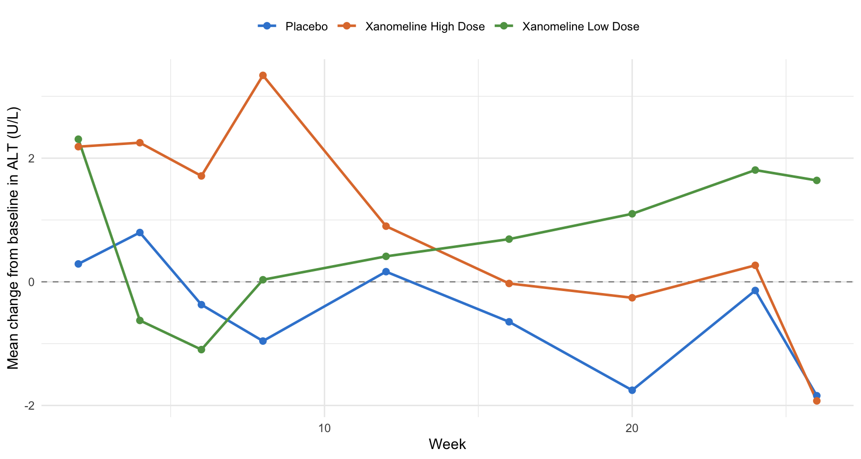
Here is where we are headed — mean change from baseline in ALT (a liver enzyme) over the study, by treatment arm, computed straight from the ADLB we derive:

That figure reads off four ADLB columns — PARAMCD, AVISIT, CHG, and TRT01A — one row per subject per test per visit. By the end of this lesson you will have derived all of them. If “ADaM”, “BDS”, or “SDTM” (the Study Data Tabulation Model — the standardized collected data ADaM is built from) are new, start with the CDISC (Clinical Data Interchange Standards Consortium) standards, which maps where ADLB sits; ADLB also reads its subject-level variables back from the ADSL you build first.

What the BDS structure is

ADSL, which you met in the ADSL lesson, has one row per subject — wide, with a column for every attribute. A findings dataset cannot work that way: a subject has a value for every lab test at every visit, far too many to be columns. So findings ADaM datasets are tall instead of wide. That tall shape is the BDS (Basic Data Structure), defined by the CDISC ADaM standard and shared by ADLB, ADVS (vital signs), and ADEG (ECG).

The BDS rule is simple: one row per subject, per parameter, per timepoint. One subject’s ALT at week 2 is a row; their ALT at week 4 is another row; their creatinine at week 2 is another row again. A single column, AVAL, holds whatever value that row measures — the analyte is named by PARAMCD, not by the column. That is what lets one dataset hold 40 different lab tests without 40 different value columns.

A handful of variables carry the structure. These are the load-bearing BDS columns this lesson derives:

Variable	Label	What it holds
PARAMCD	Parameter Code	The analyte identifier — ALT, CREAT, WBC. One value names each row’s test.
PARAM	Parameter	The human-readable parameter, e.g. Alanine Aminotransferase (U/L).
AVAL	Analysis Value	The numeric result for this parameter at this timepoint.
AVALC	Analysis Value (C)	The character result, for non-numeric findings.
AVISIT / AVISITN	Analysis Visit	The analysis visit label and its sort order.
ADT / ADY	Analysis Date / Day	The date of the measurement, and the study day relative to first dose.
ABLFL	Baseline Record Flag	"Y" on the one row that is this subject-parameter’s baseline.
BASE	Baseline Value	The baseline AVAL, copied onto every row of the subject-parameter.
CHG / PCHG	Change / % Change from Baseline	AVAL − BASE, and that change as a percent of BASE.
ANRIND	Analysis Reference Range Indicator	LOW / NORMAL / HIGH — where AVAL falls vs its reference range.
ANL01FL	Analysis Flag 01	"Y" on the records that feed a given analysis (e.g. one row per visit).

Two conventions are worth fixing up front:

• AVAL is parameter-agnostic. The same column holds ALT in U/L on one row and creatinine in µmol/L on the next. Always read AVAL together with PARAMCD — never assume a unit. That is the whole trade of the BDS: maximum flexibility, at the cost of a value column that means nothing on its own.
• Baseline is a derived flag, not a visit. ABLFL == "Y" marks the record admiral chooses as baseline (here, the last value on or before first dose). CHG and PCHG are computed against that flagged value, so the flag is the single most important derivation in the dataset.

The trial we use is the CDISC pilot study shipped in pharmaversesdtm — a synthetic, license-free parallel-arm study comparing placebo against two Xanomeline doses.

The source data

ADLB is built from the SDTM LB (Laboratory Test Results) domain plus the ADSL you derived first. LB is already in a long, one-row-per-result shape — close to BDS — so most of the work is deriving the analysis variables (dates, baseline, change) on top of it. We pull the subject-level treatment variables from ADSL.

library(admiral)
library(dplyr, warn.conflicts = FALSE)
library(pharmaversesdtm)
library(pharmaverseadam)
library(lubridate)
library(stringr)

# LB — the raw lab domain, one row per result. convert_blanks_to_na() turns
# SDTM's empty strings "" into proper NA so admiral's date/merge functions work.
lb <- pharmaversesdtm::lb %>% convert_blanks_to_na()

# ADSL — one row per subject, the treatment + demographics backbone we merge from.
adsl <- pharmaverseadam::adsl

lb %>%
  select(USUBJID, LBTESTCD, LBTEST, VISIT, LBDTC, LBSTRESN, LBSTNRLO, LBSTNRHI) %>%
  filter(LBTESTCD == "ALT", USUBJID == "01-701-1015") %>%
  head(5)

# A tibble: 5 × 8
  USUBJID     LBTESTCD LBTEST             VISIT LBDTC LBSTRESN LBSTNRLO LBSTNRHI
  <chr>       <chr>    <chr>              <chr> <chr>    <dbl>    <dbl>    <dbl>
1 01-701-1015 ALT      Alanine Aminotran… SCRE… 2013…       27        6       34
2 01-701-1015 ALT      Alanine Aminotran… WEEK… 2014…       41        6       34
3 01-701-1015 ALT      Alanine Aminotran… WEEK… 2014…       18        6       34
4 01-701-1015 ALT      Alanine Aminotran… WEEK… 2014…       26        6       34
5 01-701-1015 ALT      Alanine Aminotran… WEEK… 2014…       22        6       34

Each LB row already carries the result (LBSTRESN, the standardized numeric result), the test (LBTESTCD/LBTEST), the visit, the date (LBDTC), and the reference range (LBSTNRLO/LBSTNRHI). Our job is to turn those SDTM columns into the analysis-named BDS columns above.

Merge ADSL and derive the analysis dates

First bring the treatment variables from ADSL onto every lab record — every findings ADaM starts here, because change-from-baseline and treatment-emergent logic both key off TRTSDT (first dose). derive_vars_dt() then converts the character LBDTC into a real analysis date ADT, and derive_vars_dy() computes the study day ADY relative to first dose.

adsl_vars <- exprs(TRTSDT, TRTEDT, TRT01A, TRT01P)

adlb <- lb %>%
  # bring treatment dates + arms from ADSL onto each lab record
  derive_vars_merged(
    dataset_add = adsl,
    new_vars = adsl_vars,
    by_vars = exprs(STUDYID, USUBJID)
  ) %>%
  # ADT: the analysis date, parsed from the ISO character LBDTC
  derive_vars_dt(new_vars_prefix = "A", dtc = LBDTC) %>%
  # ADY: study day of the measurement, relative to first dose (TRTSDT)
  derive_vars_dy(reference_date = TRTSDT, source_vars = exprs(ADT))

adlb %>%
  filter(LBTESTCD == "ALT", USUBJID == "01-701-1015") %>%
  select(USUBJID, VISIT, ADT, ADY, TRTSDT) %>%
  head(5)

# A tibble: 5 × 5
  USUBJID     VISIT       ADT          ADY TRTSDT    
  <chr>       <chr>       <date>     <dbl> <date>    
1 01-701-1015 SCREENING 1 2013-12-26    -7 2014-01-02
2 01-701-1015 WEEK 2      2014-01-16    15 2014-01-02
3 01-701-1015 WEEK 4      2014-01-30    29 2014-01-02
4 01-701-1015 WEEK 6      2014-02-12    42 2014-01-02
5 01-701-1015 WEEK 8      2014-03-05    63 2014-01-02

derive_vars_dt() does the unglamorous but critical date parsing; derive_vars_dy() gives the familiar study-day count (day 1 is first dose, negative days are pre-dose screening), which is how reviewers read timing.

Set the BDS spine: PARAMCD, PARAM, and AVAL

Now name each row’s parameter and lift its value into AVAL — the three columns that make it a BDS dataset. In this lesson the lab test codes map straight across: LBTESTCD becomes PARAMCD, LBTEST becomes PARAM, and the standardized numeric result LBSTRESN becomes AVAL. (In a full production ADLB you would map these through a controlled parameter lookup so PARAMCD, PARAM, and PARAMN are governed by your metadata; the direct assignment keeps the BDS idea in focus.)

adlb <- adlb %>%
  mutate(
    PARAMCD = LBTESTCD,    # the analyte code names the row
    PARAM   = LBTEST,      # human-readable parameter
    AVAL    = LBSTRESN,    # the numeric value for THIS parameter
    AVALC   = LBSTRESC     # character value, for non-numeric findings
  )

adlb %>%
  filter(USUBJID == "01-701-1015", VISIT == "WEEK 2") %>%
  select(USUBJID, PARAMCD, PARAM, AVAL, AVALC) %>%
  head(6)

# A tibble: 6 × 5
  USUBJID     PARAMCD PARAM                       AVAL AVALC
  <chr>       <chr>   <chr>                      <dbl> <chr>
1 01-701-1015 ALB     Albumin                    39    39   
2 01-701-1015 ALP     Alkaline Phosphatase       50    50   
3 01-701-1015 ALT     Alanine Aminotransferase   41    41   
4 01-701-1015 AST     Aspartate Aminotransferase 33    33   
5 01-701-1015 BILI    Bilirubin                   8.55 8.55 
6 01-701-1015 BUN     Blood Urea Nitrogen         3.57 3.57 

That one subject, at one visit, now has several rows — one per lab test — each with the same AVAL column meaning a different analyte. That is the BDS shape made concrete: read AVAL only ever alongside PARAMCD.

Derive the analysis visit

Tables and figures group by analysis visit, not the raw SDTM VISIT string. We derive a clean AVISIT label and a numeric AVISITN for sorting, collapsing the unscheduled and screening visits to NA so they do not clutter the by-visit summaries.

adlb <- adlb %>%
  mutate(
    AVISIT = case_when(
      str_detect(VISIT, "SCREEN|UNSCHED|RETRIEVAL|AMBUL") ~ NA_character_,
      !is.na(VISIT) ~ str_to_title(VISIT)
    ),
    AVISITN = as.numeric(case_when(
      VISIT == "BASELINE" ~ "0",
      str_detect(VISIT, "WEEK") ~ str_trim(str_replace(VISIT, "WEEK", ""))
    ))
  )

adlb %>% count(VISIT, AVISIT, AVISITN)

# A tibble: 27 × 4
   VISIT               AVISIT   AVISITN     n
   <chr>               <chr>      <dbl> <int>
 1 AMBUL ECG PLACEMENT <NA>          NA     5
 2 AMBUL ECG REMOVAL   <NA>          NA    52
 3 BASELINE            Baseline       0    12
 4 RETRIEVAL           <NA>          NA    35
 5 SCREENING 1         <NA>          NA  9233
 6 UNSCHEDULED 1.1     <NA>          NA   781
 7 UNSCHEDULED 1.2     <NA>          NA   157
 8 UNSCHEDULED 1.3     <NA>          NA    73
 9 UNSCHEDULED 12.1    <NA>          NA    71
10 UNSCHEDULED 13.1    <NA>          NA    15
# ℹ 17 more rows

The scheduled WEEK n visits map to Week n with AVISITN = n; everything unscheduled becomes NA and is excluded from the analysis visits later. Deriving the visit once here means the demographic read-out, the safety table, and the figure all split on the same AVISIT.

Classify each value against its reference range (ANRIND)

A lab value is only interpretable against its reference range. ADaM stores that judgement in ANRIND, the Analysis Reference Range Indicator — LOW, NORMAL, or HIGH. admiral’s derive_var_anrind() computes it, but it expects the range in analysis columns ANRLO/ANRHI, so we copy them from the SDTM range first (LBSTNRLO/LBSTNRHI).

adlb <- adlb %>%
  mutate(
    ANRLO = LBSTNRLO,   # analysis range low  (from the SDTM normal range)
    ANRHI = LBSTNRHI    # analysis range high
  ) %>%
  derive_var_anrind()

adlb %>% count(ANRIND)

# A tibble: 4 × 2
  ANRIND     n
  <chr>  <int>
1 HIGH    1636
2 LOW      915
3 NORMAL 54108
4 <NA>    2921

adlb %>%
  filter(PARAMCD == "ALT", USUBJID == "01-701-1015") %>%
  select(USUBJID, PARAMCD, AVISIT, AVAL, ANRLO, ANRHI, ANRIND) %>%
  head(5)

# A tibble: 5 × 7
  USUBJID     PARAMCD AVISIT  AVAL ANRLO ANRHI ANRIND
  <chr>       <chr>   <chr>  <dbl> <dbl> <dbl> <chr> 
1 01-701-1015 ALT     <NA>      27     6    34 NORMAL
2 01-701-1015 ALT     Week 2    41     6    34 HIGH  
3 01-701-1015 ALT     Week 4    18     6    34 NORMAL
4 01-701-1015 ALT     Week 6    26     6    34 NORMAL
5 01-701-1015 ALT     Week 8    22     6    34 NORMAL

derive_var_anrind() reads the rule off the data: below ANRLO is LOW, above ANRHI is HIGH, in between is NORMAL, and a missing value or range gives NA. For this subject’s ALT, the week-2 value of 41 sits above the upper limit of 34, so admiral marks it HIGH — the kind of flag a safety review filters on directly.

Flag the baseline record (ABLFL)

This is the single most important derivation in any findings ADaM. Baseline is the reference each post-dose value is compared against, and the standard definition is the last non-missing value on or before first dose. We flag that record with ABLFL == "Y", one per subject per parameter, using admiral’s derive_var_extreme_flag() wrapped in restrict_derivation() so only pre-dose records are eligible.

adlb <- adlb %>%
  restrict_derivation(
    derivation = derive_var_extreme_flag,
    args = params(
      by_vars = exprs(STUDYID, USUBJID, PARAMCD),   # one baseline per subject per parameter
      order   = exprs(ADT, VISITNUM, LBSEQ),        # ... the LAST such record by date
      new_var = ABLFL,
      mode    = "last"
    ),
    filter = (!is.na(AVAL) & ADT <= TRTSDT)         # ... that is on/before first dose, non-missing
  )

adlb %>% count(ABLFL)

# A tibble: 2 × 2
  ABLFL     n
  <chr> <int>
1 Y      9159
2 <NA>  50421

adlb %>%
  filter(PARAMCD == "ALT", USUBJID == "01-701-1015", !is.na(AVAL)) %>%
  arrange(ADT) %>%
  select(USUBJID, PARAMCD, VISIT, ADT, TRTSDT, AVAL, ABLFL) %>%
  head(5)

# A tibble: 5 × 7
  USUBJID     PARAMCD VISIT       ADT        TRTSDT      AVAL ABLFL
  <chr>       <chr>   <chr>       <date>     <date>     <dbl> <chr>
1 01-701-1015 ALT     SCREENING 1 2013-12-26 2014-01-02    27 Y    
2 01-701-1015 ALT     WEEK 2      2014-01-16 2014-01-02    41 <NA> 
3 01-701-1015 ALT     WEEK 4      2014-01-30 2014-01-02    18 <NA> 
4 01-701-1015 ALT     WEEK 6      2014-02-12 2014-01-02    26 <NA> 
5 01-701-1015 ALT     WEEK 8      2014-03-05 2014-01-02    22 <NA> 

Read the three arguments as the baseline definition itself: by_vars — one baseline per subject per parameter; filter — only records on or before first dose with a value; order + mode = "last" — of those, take the latest. For this subject’s ALT, the screening record (before first dose) is flagged ABLFL == "Y"; every post-dose week is NA. Change the filter or mode and you change what “baseline” means for the whole submission — which is exactly why it lives in one auditable place.

Compute change from baseline (BASE, CHG, PCHG)

With baseline flagged, change from baseline is three declarative steps. derive_var_base() copies the flagged baseline AVAL onto every row of that subject-parameter as BASE; then derive_var_chg() computes CHG = AVAL − BASE and derive_var_pchg() computes the percent change.

adlb <- adlb %>%
  # copy the ABLFL=="Y" value onto every row of the subject-parameter
  derive_var_base(
    by_vars = exprs(STUDYID, USUBJID, PARAMCD),
    source_var = AVAL,
    new_var = BASE
  ) %>%
  derive_var_chg() %>%    # CHG  = AVAL - BASE
  derive_var_pchg()       # PCHG = 100 * (AVAL - BASE) / BASE

adlb %>%
  filter(PARAMCD == "ALT", USUBJID == "01-701-1015", !is.na(AVISIT)) %>%
  arrange(AVISITN) %>%
  select(USUBJID, AVISIT, BASE, AVAL, CHG, PCHG, ANRIND) %>%
  head(8)

# A tibble: 8 × 7
  USUBJID     AVISIT   BASE  AVAL   CHG   PCHG ANRIND
  <chr>       <chr>   <dbl> <dbl> <dbl>  <dbl> <chr> 
1 01-701-1015 Week 2     27    41    14  51.9  HIGH  
2 01-701-1015 Week 4     27    18    -9 -33.3  NORMAL
3 01-701-1015 Week 6     27    26    -1  -3.70 NORMAL
4 01-701-1015 Week 8     27    22    -5 -18.5  NORMAL
5 01-701-1015 Week 12    27    27     0   0    NORMAL
6 01-701-1015 Week 16    27    17   -10 -37.0  NORMAL
7 01-701-1015 Week 20    27    21    -6 -22.2  NORMAL
8 01-701-1015 Week 24    27    23    -4 -14.8  NORMAL

Now read one subject’s story straight off the rows: ALT starts at a baseline of 27, jumps to 41 at week 2 (CHG = +14, PCHG = +51.9%, flagged HIGH), then settles back into the normal range for the rest of the study. That single-subject narrative — value, baseline, change, range flag, across visits — is what the BDS is for, and it scales to every analyte and every subject in the same shape.

Flag the analysis records (ANL01FL)

A safety table usually wants one record per subject per parameter per visit — but a subject can have repeats (an unscheduled re-draw, a duplicate). ANL01FL marks the single record that feeds the analysis. We flag the last value per subject-parameter-visit, restricted to the scheduled analysis visits.

adlb <- adlb %>%
  restrict_derivation(
    derivation = derive_var_extreme_flag,
    args = params(
      by_vars = exprs(STUDYID, USUBJID, PARAMCD, AVISIT),  # one per subject/param/visit
      order   = exprs(ADT, AVAL),
      new_var = ANL01FL,
      mode    = "last"
    ),
    filter = !is.na(AVISITN) & !is.na(AVAL)                # scheduled visits, non-missing
  )

adlb %>% count(ANL01FL)

# A tibble: 2 × 2
  ANL01FL     n
  <chr>   <int>
1 Y       48107
2 <NA>    11473

Downstream, a by-visit lab table filters on ANL01FL == "Y" and is guaranteed one row per subject-parameter-visit — no double counting from a repeated draw. Like ABLFL, the selection rule lives in one place, so every table that uses ANL01FL selects records the same way.

Read the finished BDS dataset

The result is a conformant ADLB: tall, one row per subject per parameter per visit, with the analysis columns the BDS defines. A final look confirms the shape.

# The BDS shape: many rows per subject, the value named by PARAMCD
adlb %>%
  filter(USUBJID == "01-701-1015", AVISIT == "Week 2") %>%
  select(USUBJID, PARAMCD, AVISIT, AVAL, BASE, CHG, ANRIND, ABLFL, ANL01FL) %>%
  head(8)

# A tibble: 8 × 9
  USUBJID     PARAMCD AVISIT  AVAL  BASE    CHG ANRIND ABLFL ANL01FL
  <chr>       <chr>   <chr>  <dbl> <dbl>  <dbl> <chr>  <chr> <chr>  
1 01-701-1015 ALB     Week 2 39    38     1     NORMAL <NA>  Y      
2 01-701-1015 ALP     Week 2 50    34    16     NORMAL <NA>  Y      
3 01-701-1015 ALT     Week 2 41    27    14     HIGH   <NA>  Y      
4 01-701-1015 AST     Week 2 33    40    -7     NORMAL <NA>  Y      
5 01-701-1015 BASOLE  Week 2  0.15  0.4  -0.25  HIGH   <NA>  Y      
6 01-701-1015 BILI    Week 2  8.55 10.3  -1.71  NORMAL <NA>  Y      
7 01-701-1015 BUN     Week 2  3.57  3.57  0     NORMAL <NA>  Y      
8 01-701-1015 CA      Week 2  2.35  2.20  0.150 NORMAL <NA>  Y      

# How many parameters and how many analysis rows did we build?
adlb %>%
  summarise(
    n_rows       = n(),
    n_subjects   = n_distinct(USUBJID),
    n_parameters = n_distinct(PARAMCD)
  )

# A tibble: 1 × 3
  n_rows n_subjects n_parameters
   <int>      <int>        <int>
1  59580        254           47

One subject at one visit spans many rows — one per lab test — each sharing the AVAL/BASE/CHG machinery. That uniformity is the BDS payoff: the same derivation code, the same table programs, and the same figure templates work for every analyte, and — swapping LB for the VS or EG domain — for vital signs and ECG too. Build ADLB once and you have built the pattern for every findings dataset in the submission.

🟢 With an AI agent

Ask Prova “how do I derive a toxicity grade (ATOXGR) for my ADLB lab values with admiral’s NCI-CTCAE grading?” — it answers grounded in this pillar’s lessons, with runnable admiral code you can try on the example pharmaverse data. The runtime is the judge. Ask Prova →

Common issues

Every CHG is NA, or baseline is the wrong value. This always traces back to ABLFL. If no record is flagged ABLFL == "Y" for a subject-parameter, BASE is NA and so is every CHG. The usual cause is the baseline filter: ADT <= TRTSDT needs a real ADT (so derive_vars_dt() must run first) and a real TRTSDT merged from ADSL. If baseline looks like a post-dose value, check mode — baseline is mode = "last" of the pre-dose records, not the first record overall.

Confusing the long BDS shape with a wide one. Newcomers from a wide, one-column-per-test mindset try to read AVAL without PARAMCD and get nonsense (ALT and creatinine averaged together). In BDS, always group or filter by PARAMCD first — AVAL has no meaning on its own. If a summary looks impossible, you have almost certainly mixed parameters.

Duplicate rows inflate your counts. A subject with an unscheduled re-draw has two records at what looks like the same visit. If a table double-counts, you filtered on AVISIT but forgot ANL01FL == "Y" — that flag exists precisely to pick the single analysis record per subject-parameter-visit. Filter on it for any by-visit summary.

Frequently asked questions

NoteWhat is the BDS (Basic Data Structure) in CDISC ADaM?

The BDS is the ADaM structure for findings data — one row per subject, per parameter, per timepoint. A single AVAL column holds the value, and PARAMCD names which parameter that row measures, so one dataset can hold many different tests without a column per test. ADLB (labs), ADVS (vital signs), and ADEG (ECG) all use it. The CDISC ADaM standard defines it.

NoteHow is BDS different from ADSL’s structure?

ADSL is one row per subject — wide, with a column for every attribute. The BDS is tall — one row per subject per parameter per timepoint — because a subject has a value for every lab test at every visit, far too many to be columns. ADSL holds subject-level facts once; BDS datasets hold repeated measurements, and merge ADSL’s subject-level variables back on by USUBJID.

NoteHow do I create ADLB in R with admiral?

Start from the SDTM LB domain, merge treatment variables from ADSL, then derive the analysis date with derive_vars_dt(), set the BDS spine (PARAMCD/PARAM/AVAL), classify values against their reference range with derive_var_anrind(), flag baseline with derive_var_extreme_flag() (ABLFL), and compute change from baseline with derive_var_base(), derive_var_chg(), and derive_var_pchg(). The full sequence is worked through above and follows admiral’s BDS finding vignette.

NoteHow does admiral define baseline (ABLFL)?

Baseline is the last non-missing value on or before first dose (TRTSDT), one per subject per parameter. admiral derives it with derive_var_extreme_flag() inside restrict_derivation(): by_vars keys it per subject-parameter, the filter keeps only pre-dose non-missing records, and mode = "last" picks the latest of those. The chosen record gets ABLFL == "Y", and CHG/PCHG are computed against it.

NoteWhat is the difference between CHG and PCHG?

CHG is the absolute change from baseline, AVAL − BASE (in the parameter’s own units). PCHG is the percent change, 100 × (AVAL − BASE) / BASE. admiral derives them with derive_var_chg() and derive_var_pchg() once BASE is in place. Use CHG when the absolute amount matters and PCHG when relative movement matters or units vary widely across subjects.

NoteWhat does ANRIND mean in ADLB?

ANRIND is the Analysis Reference Range Indicator — LOW, NORMAL, or HIGH, depending on where AVAL falls relative to the reference range (ANRLO/ANRHI). admiral computes it with derive_var_anrind(). It is what safety reviews filter on to find out-of-range values, and the basis for shift tables (baseline range vs post-baseline range).

Test your understanding

ImportantYour turn: classify each value’s reference-range indicator and count out-of-range labs

Using the adlb object built in this lesson, count how many analysis records (ANL01FL == "Y") are LOW, NORMAL, or HIGH for creatinine (PARAMCD == "CREAT"), by treatment arm. Which arm has the most HIGH creatinine values?

TipHint

You already have ANRIND and ANL01FL on every row. Filter to PARAMCD == "CREAT", the analysis records (ANL01FL == "Y"), and the real treatment arms (drop "Screen Failure"), then count() by TRT01A and ANRIND. No new derivation is needed — the flags do the work.

TipSolution

adlb %>%
  filter(PARAMCD == "CREAT", ANL01FL == "Y", TRT01A != "Screen Failure") %>%
  count(TRT01A, ANRIND)

The point is conceptual: because ANRIND was derived once, the same two flags (ANRIND for the classification, ANL01FL for the analysis record) answer any out-of-range question for any parameter — you never re-derive the range logic. Swap "CREAT" for "ALT" or "K" and the same line works.

NoteQuick check: what is the defining structural rule of the BDS?

A. One row per subject B. One row per subject per parameter per timepoint C. One row per subject per visit, all parameters in columns

TipShow answer

B. The Basic Data Structure is one row per subject, per parameter, per timepoint, with the value in a single AVAL column named by PARAMCD. A is ADSL’s subject-level structure. C is the wide shape the BDS deliberately avoids — putting parameters in columns is exactly what stops a findings dataset from scaling to dozens of tests.

Conclusion

ADLB looks like a wall of rows, but it is really one idea repeated: the Basic Data Structure — one row per subject, per parameter, per timepoint, with the value in AVAL and the analyte in PARAMCD. Everything else is derivation on that spine: derive_vars_dt() for the date, derive_var_anrind() for the reference-range flag, derive_var_extreme_flag() for the baseline (ABLFL), and derive_var_base() / derive_var_chg() / derive_var_pchg() for the change-from-baseline numbers every safety lab table is built on. Get the baseline flag right and the rest follows. And because the BDS is shared, the moment you can build ADLB you can build ADVS and ADEG — same structure, same admiral moves, a different source domain. That reuse is the reason the BDS exists.

Note

This lesson is reproducible: every result on this page was produced by the code shown — copy any block and run it to reproduce them. The runtime is the judge.

Related lessons

• Create the ADSL subject-level analysis dataset — the one-row-per-subject backbone ADLB merges its treatment variables back from. · Build the adverse-events ADaM dataset (ADAE) — the OCCDS (Occurrence Data Structure) sibling, the other main findings/events shape. · Build the time-to-event ADaM dataset (ADTTE) — a specialized BDS dataset for survival endpoints. · The CDISC standards: CDASH, SDTM, ADaM, Define-XML — where ADLB and the BDS sit in the ADaM model.
• Where this fits: the regulatory and CDISC foundations → building ADaM with admiral (ADSL → ADLB and the BDS — you are here → ADAE → ADTTE) → producing the tables, listings, and figures every analysis ships. ADLB is the canonical BDS dataset every other findings dataset (ADVS, ADEG) mirrors.

Was this page helpful?

Prove you can do it. Master the whole Clinical Programming in R (pharmaverse) series — track your path, build projects, and earn a certificate.

Start free →

Go Pro — unlimited Prova on your own data and a verifiable certificate that proves the skill.

from $15/mo billed yearly

Go Pro →

✓ You're Pro — keep going. The runtime is the judge.

Get new R & Python lessons by email

Practical, reproducible, no spam. Unsubscribe anytime.

Double opt-in. We never share your email.

Share this pageXLinkedInRedditHN