ADVS in R with admiral: the Vital-Signs Analysis Dataset and Per-Timepoint Baselines

Derive a CDISC-conformant vital-signs analysis dataset (ADVS) with admiral — the BDS structure plus the analysis-timepoint (ATPT/ATPTN) and BASETYPE machinery that orthostatic blood pressure needs, so a supine baseline and a standing baseline are each computed against the right position

A complete, runnable tutorial for ADVS, the vital-signs analysis dataset, and the per-timepoint machinery a findings ADaM needs when a parameter is measured in more than one position. Recap the BDS (Basic Data Structure) from ADLB, then build a conformant ADVS in R from the SDTM VS domain with admiral: PARAMCD/AVAL from VSTESTCD/VSSTRESN, the analysis timepoint (ATPT/ATPTN) from VSTPT/VSTPTNUM, derive_basetype_records() to define a position-specific BASETYPE for orthostatic blood pressure, then derive_var_base()/derive_var_chg() within BASETYPE, plus derive_var_anrind() and the baseline (ABLFL) and analysis (ANL01FL) flags — all on public pharmaverse data, so every line runs.

TipKey takeaways

• ADVS (the vital-signs analysis dataset) is the second BDS findings dataset. It shares the BDS (Basic Data Structure) of ADLB, the lab analysis dataset — one row per subject, per parameter, per timepoint, organized around PARAMCD and AVAL — but adds one dimension ADLB does not have: the analysis timepoint.
• Vitals are measured at multiple positions. Orthostatic blood pressure is collected supine (lying down) and standing at the same visit. Those are different analysis timepoints (ATPT/ATPTN), and each needs its own baseline — a subject’s standing blood pressure must be compared to their standing baseline, not their supine one.
• derive_basetype_records() is the new machinery. It stamps a BASETYPE on every row so baseline, change from baseline, and the analysis flag are all computed within a position, not across positions.
• Everything else is the ADLB pattern, keyed on BASETYPE. derive_var_extreme_flag() for the baseline flag (ABLFL), derive_var_base() / derive_var_chg() for change from baseline, and derive_var_anrind() for the reference-range indicator — each by_vars list simply gains BASETYPE.
• Get BASETYPE right and per-position analysis is automatic. Miss it and every standing value is silently compared against a supine baseline — the single most common ADVS bug.

Introduction

Blood pressure is not measured once. In a trial that watches for orthostatic effects — a drop in blood pressure on standing that a drug can cause or worsen — vital signs are collected in more than one position at the same visit: supine (lying down) first, then standing after one minute and after three. The same subject, the same visit, the same parameter, three readings. And each position has its own normal level: standing blood pressure is typically lower than supine, so a subject’s standing value can only be judged against their standing baseline.

That is the wrinkle ADVS — the vital-signs analysis dataset — adds to the findings ADaM (Analysis Data Model) you already know. In the ADLB lesson you built the BDS (Basic Data Structure) — the tall shape the CDISC ADaM standard defines: one row per subject, per parameter, per timepoint, with the value in AVAL and the analyte named by PARAMCD. ADLB had no positions to worry about — a lab draw is a lab draw — so a single baseline per subject-parameter was correct. ADVS carries the analysis timepoint, and with it the need for a per-position baseline. This lesson teaches that machinery: admiral’s derive_basetype_records() and the BASETYPE variable it creates.

We build a conformant ADVS in R with admiral, the pharmaverse package for ADaM derivation, on public pharmaverse example data, following admiral’s Creating a BDS Finding ADaM vignette — which is built on vital signs precisely because it is where the timepoint dimension lives.

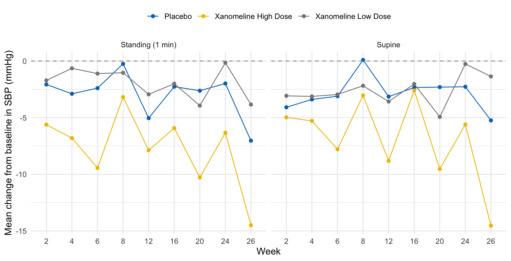
Here is where we are headed — mean change from baseline in systolic blood pressure (SBP) over the study, by treatment arm, split by position, computed straight from the ADVS we derive:

That figure reads off four ADVS columns — PARAMCD, AVISIT, CHG, and the position behind each BASETYPE — and it splits by position because the change is computed within position. By the end of this lesson you will have derived all of it. If BDS, ADaM, or SDTM (the Study Data Tabulation Model — the standardized collected data ADaM is built from) are new, start with the ADLB lesson and the BDS structure; ADVS reuses every move it teaches and adds one.

What ADVS adds to the BDS: the timepoint dimension

ADVS is a BDS dataset, so the spine is the same as ADLB’s — one row per subject, per parameter, per timepoint, with PARAMCD naming the parameter and AVAL holding its value. What is new is that a vital-signs parameter can be measured several times at one visit, in different body positions, so the “timepoint” is no longer just the visit. Two variables carry that, and one derived variable makes it usable:

Variable	Label	What it holds
PARAMCD / PARAM	Parameter Code / Parameter	The vital sign — SYSBP, DIABP, PULSE, TEMP. (Same as ADLB.)
AVAL	Analysis Value	The numeric result for this parameter at this timepoint. (Same as ADLB.)
AVISIT / AVISITN	Analysis Visit	The analysis visit label and its sort order. (Same as ADLB.)
ATPT / ATPTN	Analysis Timepoint / (N)	New. The within-visit timepoint — “AFTER LYING DOWN FOR 5 MINUTES” (supine) vs “AFTER STANDING FOR 1 MINUTE” — and its numeric code.
ABLFL	Baseline Record Flag	"Y" on the one baseline row per position for this subject-parameter.
BASE / CHG / PCHG	Baseline / Change / % Change	The baseline value and the change from it — computed within the position.
ANRIND	Analysis Reference Range Indicator	LOW / NORMAL / HIGH for this value vs its reference range. (Same as ADLB.)
ANL01FL	Analysis Flag 01	"Y" on the one record that feeds a given analysis, per position per visit.
BASETYPE	Baseline Type	The key new variable. Names the group of records that share a baseline — one per position. Every baseline-dependent derivation keys on it.

The whole difference between ADLB and ADVS lives in one word: position. ADLB flags one baseline per subject-parameter. ADVS must flag one baseline per subject-parameter-per-position, because a supine reading and a standing reading measured minutes apart are not comparable. The mechanism admiral gives you for that is BASETYPE — a label you attach to each record naming the baseline group it belongs to. Once every row carries a BASETYPE, the same admiral functions you used for ADLB do the per-position work automatically, just by adding BASETYPE to their by_vars.

The trial we use is the CDISC (Clinical Data Interchange Standards Consortium) pilot study shipped in pharmaversesdtm — a synthetic, license-free parallel-arm study comparing placebo against two Xanomeline doses, whose vital signs are collected at exactly these orthostatic timepoints.

The source data

ADVS is built from the SDTM VS (Vital Signs) domain plus the ADSL (Subject-Level Analysis Dataset) — the one-row-per-subject backbone you derived first, from which every findings ADaM reads its treatment variables. VS is already long, one row per result, and it carries the timepoint (VSTPT/VSTPTNUM) and position (VSPOS) that make ADVS interesting.

library(admiral)
library(dplyr, warn.conflicts = FALSE)
library(pharmaversesdtm)
library(pharmaverseadam)
library(lubridate)
library(stringr)
library(tibble)

# VS — the raw vital-signs domain, one row per result. convert_blanks_to_na()
# turns SDTM's empty strings "" into proper NA so admiral's functions work.
vs <- pharmaversesdtm::vs %>% convert_blanks_to_na()

# ADSL — one row per subject, the treatment + demographics backbone we merge from.
adsl <- pharmaverseadam::adsl

# The timepoint/position structure that makes ADVS different from ADLB:
vs %>% count(VSTPTNUM, VSTPT, VSPOS)

# A tibble: 4 × 4
  VSTPTNUM VSTPT                          VSPOS        n
     <dbl> <chr>                          <chr>    <int>
1      815 AFTER LYING DOWN FOR 5 MINUTES SUPINE    8208
2      816 AFTER STANDING FOR 1 MINUTE    STANDING  8204
3      817 AFTER STANDING FOR 3 MINUTES   STANDING  8207
4       NA <NA>                           <NA>      5024

Read that table: each blood-pressure and pulse reading is taken at one of three timepoints — after lying down 5 minutes (VSTPTNUM == 815, the supine position), after standing 1 minute (816), and after standing 3 minutes (817) — while height, weight, and temperature have no timepoint (NA). Those numeric timepoint codes are what we will turn into positions and, from them, per-position baselines.

Merge ADSL and derive the analysis date

Every findings ADaM starts by bringing the treatment variables from ADSL onto each record, because baseline logic keys off TRTSDT (the first-dose date). derive_vars_dt() then converts the character VSDTC into a real analysis date ADT.

adsl_vars <- exprs(TRTSDT, TRTEDT, TRT01A, TRT01P)

advs <- vs %>%
  # bring treatment dates + arms from ADSL onto each vital-signs record
  derive_vars_merged(
    dataset_add = adsl,
    new_vars = adsl_vars,
    by_vars = exprs(STUDYID, USUBJID)
  ) %>%
  # ADT: the analysis date, parsed from the ISO character VSDTC
  derive_vars_dt(new_vars_prefix = "A", dtc = VSDTC) %>%
  # ADY: study day of the measurement, relative to first dose (TRTSDT)
  derive_vars_dy(reference_date = TRTSDT, source_vars = exprs(ADT))

advs %>%
  filter(VSTESTCD == "SYSBP", USUBJID == "01-701-1015") %>%
  select(USUBJID, VISIT, VSTPT, ADT, ADY, TRTSDT) %>%
  head(4)

# A tibble: 4 × 6
  USUBJID     VISIT       VSTPT                      ADT          ADY TRTSDT    
  <chr>       <chr>       <chr>                      <date>     <dbl> <date>    
1 01-701-1015 SCREENING 1 AFTER LYING DOWN FOR 5 MI… 2013-12-26    -7 2014-01-02
2 01-701-1015 SCREENING 1 AFTER STANDING FOR 1 MINU… 2013-12-26    -7 2014-01-02
3 01-701-1015 SCREENING 1 AFTER STANDING FOR 3 MINU… 2013-12-26    -7 2014-01-02
4 01-701-1015 SCREENING 2 AFTER LYING DOWN FOR 5 MI… 2013-12-31    -2 2014-01-02

ADT is the date the derivations below compare against TRTSDT; ADY is the familiar study day (day 1 is first dose, negative days are pre-dose screening), which is how reviewers read timing.

Set the BDS spine: PARAMCD, PARAM, and AVAL

Now name each row’s parameter and lift its value into AVAL. We map the vital-signs test codes to analysis parameters through a small lookup table — derive_vars_merged_lookup() joins it on VSTESTCD, giving a governed PARAMCD and human-readable PARAM — then set AVAL from the standardized numeric result VSSTRESN.

# One controlled place that maps each SDTM test code to its analysis parameter.
param_lookup <- tibble::tribble(
  ~VSTESTCD, ~PARAMCD,                            ~PARAM,
  "HEIGHT",  "HEIGHT",                     "Height (cm)",
  "WEIGHT",  "WEIGHT",                     "Weight (kg)",
  "DIABP",    "DIABP", "Diastolic Blood Pressure (mmHg)",
  "PULSE",    "PULSE",          "Pulse Rate (beats/min)",
  "SYSBP",    "SYSBP",  "Systolic Blood Pressure (mmHg)",
  "TEMP",      "TEMP",                 "Temperature (C)"
)

advs <- advs %>%
  derive_vars_merged_lookup(
    dataset_add = param_lookup,
    new_vars = exprs(PARAMCD, PARAM),
    by_vars = exprs(VSTESTCD)
  ) %>%
  mutate(AVAL = VSSTRESN)   # the numeric value for THIS parameter

advs %>%
  filter(USUBJID == "01-701-1015", VISIT == "WEEK 2", VSTPTNUM == 815) %>%
  select(USUBJID, PARAMCD, PARAM, VSTPT, AVAL) %>%
  head(6)

# A tibble: 3 × 5
  USUBJID     PARAMCD PARAM                           VSTPT                 AVAL
  <chr>       <chr>   <chr>                           <chr>                <dbl>
1 01-701-1015 DIABP   Diastolic Blood Pressure (mmHg) AFTER LYING DOWN FO…    56
2 01-701-1015 PULSE   Pulse Rate (beats/min)          AFTER LYING DOWN FO…    58
3 01-701-1015 SYSBP   Systolic Blood Pressure (mmHg)  AFTER LYING DOWN FO…   114

Using a lookup rather than a bare PARAMCD = VSTESTCD is how a production ADVS keeps its parameters governed by metadata — the same code, label, and ordering every table uses. AVAL is now parameter-agnostic: read it only ever together with PARAMCD, exactly as in ADLB.

Derive the analysis visit and the analysis timepoint

Here is the step ADLB did not have. Alongside the analysis visit (AVISIT/AVISITN), we derive the analysis timepoint (ATPT/ATPTN) straight from the SDTM VSTPT/VSTPTNUM. That timepoint is what distinguishes a supine reading from a standing one at the same visit.

advs <- advs %>%
  mutate(
    AVISIT = case_when(
      str_detect(VISIT, "SCREEN|UNSCHED|RETRIEVAL|AMBUL") ~ NA_character_,
      !is.na(VISIT) ~ str_to_title(VISIT)
    ),
    AVISITN = as.numeric(case_when(
      VISIT == "BASELINE" ~ "0",
      str_detect(VISIT, "WEEK") ~ str_trim(str_replace(VISIT, "WEEK", ""))
    )),
    ATPT  = VSTPT,       # the within-visit timepoint label (position, here)
    ATPTN = VSTPTNUM     # its numeric code, for sorting and BASETYPE
  )

advs %>% count(ATPTN, ATPT)

# A tibble: 4 × 3
  ATPTN ATPT                               n
  <dbl> <chr>                          <int>
1   815 AFTER LYING DOWN FOR 5 MINUTES  8208
2   816 AFTER STANDING FOR 1 MINUTE     8204
3   817 AFTER STANDING FOR 3 MINUTES    8207
4    NA <NA>                            5024

AVISIT collapses the unscheduled and screening visits to NA, exactly as in ADLB, so they do not clutter by-visit summaries. ATPT/ATPTN carry the orthostatic structure through the dataset: three real timepoints for blood pressure and pulse, NA for the once-per-visit measurements. Everything from here keys off ATPTN.

Classify each value against its reference range (ANRIND)

A vital sign is judged against a reference range just like a lab value. ADaM stores that in ANRIND (the Analysis Reference Range Indicator): LOW, NORMAL, or HIGH. derive_var_anrind() computes it, reading the range from analysis columns ANRLO/ANRHI, so we merge a small per-parameter range table first.

# Per-parameter reference ranges (the study's analysis ranges).
range_lookup <- tibble::tribble(
  ~PARAMCD, ~ANRLO, ~ANRHI,
  "SYSBP",      90,    130,
  "DIABP",      60,     80,
  "PULSE",      60,    100,
  "TEMP",     36.5,   37.5
)

advs <- advs %>%
  derive_vars_merged(dataset_add = range_lookup, by_vars = exprs(PARAMCD)) %>%
  derive_var_anrind()

advs %>%
  filter(PARAMCD == "SYSBP", USUBJID == "01-701-1015", VISIT == "WEEK 8") %>%
  select(USUBJID, PARAMCD, ATPT, AVAL, ANRLO, ANRHI, ANRIND) %>%
  head(3)

# A tibble: 3 × 7
  USUBJID     PARAMCD ATPT                            AVAL ANRLO ANRHI ANRIND
  <chr>       <chr>   <chr>                          <dbl> <dbl> <dbl> <chr> 
1 01-701-1015 SYSBP   AFTER LYING DOWN FOR 5 MINUTES   138    90   130 HIGH  
2 01-701-1015 SYSBP   AFTER STANDING FOR 1 MINUTE      146    90   130 HIGH  
3 01-701-1015 SYSBP   AFTER STANDING FOR 3 MINUTES     140    90   130 HIGH  

derive_var_anrind() reads the rule off the data: below ANRLO is LOW, above ANRHI is HIGH, in between is NORMAL. The same range applies across positions here, but the indicator is computed row by row — so a standing value can read HIGH while the supine value at the same visit reads NORMAL.

Define the baseline type per position (BASETYPE) — the key step

This is the derivation that makes ADVS more than ADLB. Because a subject has a supine baseline and a standing baseline for the same parameter, we cannot flag “the” baseline record — we must flag one per position. admiral’s derive_basetype_records() makes that possible: it assigns a BASETYPE label to every row, naming the group of records that share a baseline. We define one BASETYPE per timepoint code, plus a catch-all "LAST" for the parameters that have no timepoint.

advs <- advs %>%
  derive_basetype_records(
    basetypes = exprs(
      "LAST: AFTER LYING DOWN FOR 5 MINUTES" = ATPTN == 815,   # supine
      "LAST: AFTER STANDING FOR 1 MINUTE"    = ATPTN == 816,   # standing, 1 min
      "LAST: AFTER STANDING FOR 3 MINUTES"   = ATPTN == 817,   # standing, 3 min
      "LAST"                                  = is.na(ATPTN)     # height/weight/temp
    )
  )

advs %>% count(ATPT, ATPTN, BASETYPE)

# A tibble: 4 × 4
  ATPT                           ATPTN BASETYPE                                n
  <chr>                          <dbl> <chr>                               <int>
1 AFTER LYING DOWN FOR 5 MINUTES   815 LAST: AFTER LYING DOWN FOR 5 MINUT…  8208
2 AFTER STANDING FOR 1 MINUTE      816 LAST: AFTER STANDING FOR 1 MINUTE    8204
3 AFTER STANDING FOR 3 MINUTES     817 LAST: AFTER STANDING FOR 3 MINUTES   8207
4 <NA>                              NA LAST                                 5024

Read the basetypes list as the definition of what shares a baseline: each condition selects a set of records, and every matched record gets that BASETYPE. Supine records will get a supine baseline, standing-at-1-minute records a standing-at-1-minute baseline, and so on. The once-per-visit parameters (height, weight, temperature) have no timepoint, so they fall into the plain "LAST" group. Nothing is compared yet — BASETYPE just labels the groups; the next three steps do the per-group work simply by including BASETYPE in their by_vars.

Flag the baseline record per position (ABLFL)

Now flag the baseline the same way ADLB did — the last non-missing value on or before first dose — but within each BASETYPE. Adding BASETYPE to by_vars is the whole change: it turns “one baseline per subject-parameter” into “one baseline per subject-parameter-per-position.”

advs <- advs %>%
  restrict_derivation(
    derivation = derive_var_extreme_flag,
    args = params(
      by_vars = exprs(STUDYID, USUBJID, BASETYPE, PARAMCD),  # ... now PER position
      order   = exprs(ADT, ATPTN, VISITNUM),
      new_var = ABLFL,
      mode    = "last"
    ),
    filter = (!is.na(AVAL) & ADT <= TRTSDT & !is.na(BASETYPE))
  )

advs %>% count(ABLFL)

# A tibble: 2 × 2
  ABLFL     n
  <chr> <int>
1 Y      3048
2 <NA>  26595

by_vars now reads: one baseline per subject, per BASETYPE, per parameter — so a subject’s supine SYSBP and standing SYSBP each get their own ABLFL == "Y" record. The filter (non-missing value, on or before first dose) and mode = "last" are unchanged from ADLB. This one added by_vars entry is the difference between a correct ADVS and one where every standing value is compared against a supine baseline.

Compute change from baseline within position (BASE, CHG, PCHG)

With baseline flagged per position, change from baseline is the ADLB sequence with BASETYPE added to derive_var_base(). derive_var_base() copies each BASETYPE’s flagged baseline onto every row of that position; then derive_var_chg() and derive_var_pchg() compute the absolute and percent change.

advs <- advs %>%
  derive_var_base(
    by_vars = exprs(STUDYID, USUBJID, PARAMCD, BASETYPE),   # copy the per-position baseline
    source_var = AVAL,
    new_var = BASE
  ) %>%
  derive_var_chg() %>%    # CHG  = AVAL - BASE
  derive_var_pchg()       # PCHG = 100 * (AVAL - BASE) / BASE

advs %>%
  filter(PARAMCD == "SYSBP", USUBJID == "01-701-1015",
         AVISIT %in% c("Baseline", "Week 8"), ATPTN %in% c(815, 816)) %>%
  arrange(ATPTN, AVISITN) %>%
  select(AVISIT, ATPT, BASE, AVAL, CHG, ANRIND) %>%
  head(4)

# A tibble: 4 × 6
  AVISIT   ATPT                            BASE  AVAL   CHG ANRIND
  <chr>    <chr>                          <dbl> <dbl> <dbl> <chr> 
1 Baseline AFTER LYING DOWN FOR 5 MINUTES   130   130     0 NORMAL
2 Week 8   AFTER LYING DOWN FOR 5 MINUTES   130   138     8 HIGH  
3 Baseline AFTER STANDING FOR 1 MINUTE      121   121     0 NORMAL
4 Week 8   AFTER STANDING FOR 1 MINUTE      121   146    25 HIGH  

Because derive_var_base() keyed on BASETYPE, this subject’s supine rows carry a supine BASE and the standing rows carry a standing BASE — different numbers, as they should be. The week-8 supine change is measured against the supine baseline, the week-8 standing change against the standing baseline. That is the payoff of BASETYPE: change from baseline is honest per position, with no extra bookkeeping.

Flag the analysis records per position (ANL01FL)

A safety table usually wants one record per subject, per parameter, per visit — but now per position too. ANL01FL marks it, and like ABLFL it simply gains BASETYPE in its by_vars.

advs <- advs %>%
  restrict_derivation(
    derivation = derive_var_extreme_flag,
    args = params(
      by_vars = exprs(STUDYID, USUBJID, BASETYPE, PARAMCD, AVISIT),  # per position, per visit
      order   = exprs(ADT, ATPTN, AVAL),
      new_var = ANL01FL,
      mode    = "last"
    ),
    filter = !is.na(AVISITN)     # scheduled analysis visits
  )

advs %>% count(ANL01FL)

# A tibble: 2 × 2
  ANL01FL     n
  <chr>   <int>
1 Y       19783
2 <NA>     9860

Downstream, a by-visit vital-signs table filters on ANL01FL == "Y" and is guaranteed one row per subject-parameter-visit-position — the supine and standing readings kept separate, no double counting from a repeated draw.

Read one subject’s per-position story

The result is a conformant ADVS: tall, BDS-shaped, with a per-position baseline attached to every row. Read a single subject’s systolic blood pressure across positions and visits and the whole point of BASETYPE is visible at once.

advs %>%
  filter(PARAMCD == "SYSBP", USUBJID == "01-701-1015",
         AVISIT %in% c("Baseline", "Week 2", "Week 8"), !is.na(ATPTN)) %>%
  arrange(ATPTN, AVISITN) %>%
  select(AVISIT, ATPT, BASE, AVAL, CHG, ANRIND, ABLFL) %>%
  as.data.frame()

    AVISIT                           ATPT BASE AVAL CHG ANRIND ABLFL
1 Baseline AFTER LYING DOWN FOR 5 MINUTES  130  130   0 NORMAL     Y
2   Week 2 AFTER LYING DOWN FOR 5 MINUTES  130  114 -16 NORMAL  <NA>
3   Week 8 AFTER LYING DOWN FOR 5 MINUTES  130  138   8   HIGH  <NA>
4 Baseline    AFTER STANDING FOR 1 MINUTE  121  121   0 NORMAL     Y
5   Week 2    AFTER STANDING FOR 1 MINUTE  121  121   0 NORMAL  <NA>
6   Week 8    AFTER STANDING FOR 1 MINUTE  121  146  25   HIGH  <NA>
7 Baseline   AFTER STANDING FOR 3 MINUTES  131  131   0   HIGH     Y
8   Week 2   AFTER STANDING FOR 3 MINUTES  131  132   1   HIGH  <NA>
9   Week 8   AFTER STANDING FOR 3 MINUTES  131  140   9   HIGH  <NA>

Three positions, three baselines: supine baseline 130, standing-at-1-minute 121, standing-at-3-minutes 131 — the same subject, same parameter, same baseline visit, yet three different BASE values because position matters. Each post-baseline CHG is computed against the baseline for its own position. Had we flagged a single baseline across positions (the ADLB approach), the standing values would have been measured against 130 instead of 121 — a 9 mmHg error injected into every standing change, and exactly the mistake BASETYPE exists to prevent.

🟢 With an AI agent

Ask Prova “how do I add a worst-case post-baseline flag (WORSTFL) per position to my ADVS with admiral’s slice_derivation()?” — it answers grounded in this pillar’s lessons, with runnable admiral code you can try on the example pharmaverse data. The runtime is the judge. Ask Prova →

Common issues

Every standing value is compared against the supine baseline. This is the ADVS bug, and it happens whenever BASETYPE is missing from the baseline machinery. If you flag ABLFL and copy BASE with by_vars = exprs(STUDYID, USUBJID, PARAMCD) — the ADLB keys — admiral picks one baseline across all positions, and every standing CHG is wrong by the supine-standing gap. The fix is to run derive_basetype_records() first and add BASETYPE to the by_vars of derive_var_extreme_flag() (for ABLFL) and derive_var_base(). If a subject’s supine and standing baselines come out identical when they should differ, this is why.

A parameter with no timepoint gets no baseline. Height, weight, and temperature have ATPTN == NA, so they only get a BASETYPE if your basetypes list includes a catch-all condition like "LAST" = is.na(ATPTN). Leave it out and those rows have BASETYPE == NA, the filter = !is.na(BASETYPE) drops them from ABLFL, and their BASE/CHG come back NA. Always give the timepoint-less parameters a BASETYPE group.

Duplicate positions inflate a by-visit count. A subject measured supine and standing at one visit has (at least) two SYSBP rows there. If a table double-counts, you filtered on AVISIT but forgot to keep the positions separate — filter on ANL01FL == "Y" (which is per-position) or group by ATPTN/BASETYPE, never AVISIT alone, for any by-visit vital-signs summary.

Frequently asked questions

NoteWhat is ADVS in CDISC ADaM?

ADVS is the vital-signs analysis dataset — a findings ADaM built on the BDS (Basic Data Structure), one row per subject, per parameter (PARAMCD = SYSBP, DIABP, PULSE, TEMP…), per timepoint, with the value in AVAL. It adds an analysis-timepoint dimension (ATPT/ATPTN) that ADLB does not have, because vital signs like orthostatic blood pressure are measured in more than one position at a visit. You build it from the SDTM VS domain with admiral, following the BDS finding vignette.

NoteWhat is BASETYPE in ADaM, and when do I need it?

BASETYPE is an ADaM variable that names the group of records sharing a baseline. You need it whenever a subject-parameter has more than one baseline — most commonly vital signs measured in several positions (supine vs standing for orthostatic blood pressure), where a standing value must be compared to a standing baseline, not a supine one. admiral assigns it with derive_basetype_records(); you then add BASETYPE to the by_vars of the baseline flag and change-from-baseline derivations so each position is handled separately. ADLB, whose lab draws have no positions, does not need it.

NoteHow does derive_basetype_records() work?

derive_basetype_records() takes a basetypes list of named conditions — for example "LAST: AFTER STANDING FOR 1 MINUTE" = ATPTN == 816 — and stamps the matching name onto each record as BASETYPE. A record can match more than one condition (it is then duplicated, once per matched BASETYPE), which is how one physical reading can serve as the baseline reference for several analysis groupings. Every baseline-dependent derivation downstream keys on BASETYPE.

NoteWhat is the difference between ADVS and ADLB?

Both are BDS findings datasets built with the same admiral functions, and both derive baseline (ABLFL), change from baseline (CHG/PCHG), and the reference-range indicator (ANRIND). The difference is the analysis timepoint: ADLB (labs) has one measurement per parameter per visit, so one baseline per subject-parameter is correct. ADVS (vital signs) can have several readings per visit at different positions (ATPT/ATPTN), so it needs a BASETYPE and a baseline per position. Learn ADLB first — ADVS is that pattern plus the timepoint dimension.

NoteWhat are ATPT and ATPTN in ADVS?

ATPT is the Analysis Timepoint — the within-visit timepoint description, such as “AFTER LYING DOWN FOR 5 MINUTES” or “AFTER STANDING FOR 1 MINUTE” — and ATPTN is its numeric code, used for sorting and to define BASETYPE. They typically map straight from the SDTM VSTPT/VSTPTNUM. For orthostatic assessments the timepoint effectively encodes body position, which is why the per-timepoint baseline (via BASETYPE) is the crux of an ADVS derivation.

Test your understanding

ImportantYour turn: compare a subject’s supine and standing baselines

Using the advs object built in this lesson, show the baseline records (ABLFL == "Y") for diastolic blood pressure (PARAMCD == "DIABP") for subject "01-701-1015", one per position. Are the supine and standing baseline values the same or different — and why does that matter?

TipHint

Every baseline record is already flagged. Filter to PARAMCD == "DIABP", USUBJID == "01-701-1015", and ABLFL == "Y", then select BASETYPE, ATPT, and BASE (or AVAL). No new derivation is needed — BASETYPE and ABLFL did the work.

advs %>%
  filter(PARAMCD == "DIABP", USUBJID == "01-701-1015", ABLFL == "Y") %>%
  select(BASETYPE, ATPT, AVAL, BASE)

TipSolution

advs %>%
  filter(PARAMCD == "DIABP", USUBJID == "01-701-1015", ABLFL == "Y") %>%
  arrange(ATPTN) %>%
  select(BASETYPE, ATPT, AVAL, BASE)

There is one baseline row per position, and their values differ — the supine baseline is not the standing baseline. That matters because CHG and PCHG are computed against BASE: if both positions shared one baseline, every standing change would be measured from the wrong reference. Because we keyed ABLFL and BASE on BASETYPE, each position’s change is correct. Swap "DIABP" for "SYSBP" or "PULSE" and the same per-position structure holds.

NoteQuick check: why does ADVS need BASETYPE when ADLB does not?

A. Because vital signs have more parameters than labs B. Because a vital-signs parameter can be measured at several positions in one visit, each needing its own baseline C. Because ADVS uses a different value column than AVAL

TipShow answer

B. Orthostatic vital signs are measured supine and standing at the same visit, so a subject-parameter has more than one baseline. BASETYPE names those per-position groups so baseline (ABLFL), BASE, and change from baseline are computed within a position. A is irrelevant — parameter count does not change the structure. C is false: ADVS uses AVAL and the BDS shape exactly like ADLB. The one real difference is the per-position baseline.

Conclusion

ADVS is ADLB plus one idea: a baseline per position. The BDS spine is identical — one row per subject, per parameter, per timepoint, value in AVAL, analyte in PARAMCD — and the same admiral functions derive the reference-range flag (derive_var_anrind()), the baseline (derive_var_extreme_flag() → ABLFL), and change from baseline (derive_var_base() / derive_var_chg() / derive_var_pchg()). What ADVS adds is the analysis timepoint (ATPT/ATPTN) and, from it, derive_basetype_records(), which stamps a BASETYPE on every row so all of those derivations run within a position. Add BASETYPE to the by_vars and orthostatic blood pressure — supine versus standing — is handled correctly with no extra machinery. Miss it and you compare every standing value against a supine baseline. Get BASETYPE right, and the rest is the ADLB pattern you already know.

Note

This lesson is reproducible: every result on this page was produced by the code shown — copy any block and run it to reproduce them. The runtime is the judge.

Related lessons

• ADLB in R with admiral and the BDS structure — the first findings ADaM and the Basic Data Structure ADVS reuses; start here if the BDS is new. · Create the ADSL subject-level analysis dataset — the one-row-per-subject backbone ADVS merges its treatment variables back from. · Build the adverse-events ADaM dataset (ADAE) — the OCCDS (Occurrence Data Structure) sibling, the events counterpart to the findings BDS. · The CDISC standards: CDASH, SDTM, ADaM, Define-XML — where ADVS and the BDS sit in the ADaM model.
• Where this fits: the regulatory and CDISC foundations → building ADaM with admiral (ADSL → ADLB → ADVS — you are here → ADAE → ADTTE) → producing the tables, listings, and figures every analysis ships. ADVS extends the ADLB BDS pattern with the per-timepoint baselines vital signs need.

Was this page helpful?

Prove you can do it. Master the whole Clinical Programming in R (pharmaverse) series — track your path, build projects, and earn a certificate.

Start free →

Go Pro — unlimited Prova on your own data and a verifiable certificate that proves the skill.

from $15/mo billed yearly

Go Pro →

✓ You're Pro — keep going. The runtime is the judge.

Get new R & Python lessons by email

Practical, reproducible, no spam. Unsubscribe anytime.

Double opt-in. We never share your email.

Share this pageXLinkedInRedditHN