The Efficacy Table in R: ANCOVA and LS Means with rtables and tern

Q: What is an efficacy table in a clinical trial?

It is the table that reports the trial’s primary (or key secondary) endpoint result — the formal answer to did the treatment work? For a continuous endpoint it is an ANCOVA (analysis of covariance) of the change from baseline: per treatment arm it shows the number of subjects and the adjusted (least-squares) mean change, then, for each active arm versus the reference, the difference in adjusted means with a 95% CI and p-value, adjusting for the baseline value. It sits in section 14.2 of a Clinical Study Report, whose structure follows the ICH E3 guideline.

Q: How do I build an ANCOVA table in R with rtables and tern?

Use summarize_ancova(): basic_table() |> split_cols_by("TRT01A", ref_group = "Placebo") |> add_colcounts() |> summarize_ancova(vars = "CHG", variables = list(arm = "TRT01A", covariates = "BASE"), conf_level = 0.95), then apply it with build_table(df = anl). tern fits lm(CHG ~ TRT01A + BASE), extracts the least-squares means with emmeans, and lays out n, the adjusted mean, the difference, the CI, and the p-value. The full build is worked through above on public pharmaverse data.

Q: What are LS means (least-squares means) and how do they differ from raw means?

A least-squares mean (also called an estimated marginal mean) is a model-based estimate of an arm’s mean at a common value of the covariates — here, the mean change from baseline if every arm had the same average baseline. A raw mean just averages the observed values in the arm. They coincide only when the covariate is perfectly balanced across arms; when baseline differs (as it usually does), the LS mean is the fair, adjusted estimate and the raw mean is not. The efficacy table always reports the LS mean.

Q: How do I read the adjusted mean difference and its confidence interval?

The difference in adjusted means is the active arm’s LS mean minus the reference arm’s LS mean — the estimated treatment effect on the endpoint, in the endpoint’s units. Its 95% CI is the range of effects compatible with the data: if the interval excludes 0 the effect is statistically significant (equivalently p < 0.05); if it includes 0, as in this lesson’s table, there is no significant difference from the reference. Always read the CI, not just the p-value — its width tells you how precise the estimate is.

Q: ANCOVA or MMRM for the efficacy analysis?

ANCOVA analyzes a single timepoint (e.g. the end-of-treatment visit) as change from baseline adjusted for baseline — simple, and what this lesson builds. MMRM (mixed model for repeated measures) analyzes all post-baseline visits jointly, keeps subjects with partial follow-up, and models the within-subject correlation, so it makes weaker missing-data assumptions and is the primary-analysis default in many recent trials. The reporting table looks the same (LS means, a difference, a CI, a p); the model is fitted with the mmrm package and tabulated with tern.mmrm. Learn ANCOVA first — the pattern transfers directly.

Build the primary efficacy result of a Clinical Study Report — the analysis of covariance (ANCOVA) of change from baseline, with the least-squares mean per arm and the adjusted treatment difference, 95% CI, and p-value — using tern’s summarize_ancova on public pharmaverse data

Pharma & Clinical

A complete, runnable tutorial for the clinical efficacy analysis table — the ANCOVA (analysis of covariance) table that reports the primary endpoint of a Clinical Study Report. Learn what the table shows (per-arm n, the adjusted or least-squares (LS) mean change from baseline with its standard error, and the treatment-versus-reference difference in LS means with a 95% CI and p-value, adjusting for the baseline value), then build it with rtables and tern: basic_table() |> split_cols_by(arm, ref_group=) |> summarize_ancova(vars, variables = list(arm=, covariates=), conf_level=) — on public pharmaverseadam ADVS data, so every line runs. Includes the LS-means-vs-raw-means distinction, the reference-arm choice, and why baseline enters as a covariate.

Published

July 1, 2026

Modified

July 7, 2026

Key takeaways

The efficacy table is the primary-endpoint result of a Clinical Study Report — the formal answer to did the drug work? For a continuous endpoint it is an analysis of covariance (ANCOVA) of the change from baseline, comparing each treatment arm with the reference arm while adjusting for the baseline value.
It reports adjusted, not raw, means. Each arm’s cell is the least-squares (LS) mean — the mean change you would expect if the arms had the same average baseline — with its standard error. The comparison line is the difference in LS means, its 95% confidence interval (CI), and a p-value.
Baseline is a covariate, not the outcome. The endpoint is CHG (change from baseline); BASE (the baseline value) goes on the right of the model as an adjustment. Putting baseline on the outcome side is a classic error.
One tern function builds it. summarize_ancova() fits the linear model, extracts the LS means with emmeans, and lays the result out — n, adjusted mean, difference, CI, p — inside an rtables layout.
The reference arm is the first factor level. split_cols_by("TRT01A", ref_group = "Placebo") fixes placebo as the comparator; every difference is arm minus placebo.

Introduction

The demographic table says who was in the trial and the adverse-event table says whether it was safe. The efficacy table answers the question the trial was run to answer: did the treatment work? It is the primary-endpoint analysis of a Clinical Study Report (CSR) — and for a continuous endpoint measured before and after treatment, that analysis is almost always an analysis of covariance (ANCOVA) of the change from baseline.

The table is compact but dense. For each treatment arm it gives the number of subjects analyzed and the adjusted (least-squares) mean change from baseline; then, for each active arm against the reference, the difference in adjusted means with its 95% confidence interval (CI) and p-value. “Adjusted” is the whole point: the comparison is made as if every arm had started from the same baseline, so a chance imbalance in baseline severity cannot masquerade as a treatment effect.

This is a table in the pharma TLF (tables, listings, and figures) workflow, built from one analysis dataset: a BDS (Basic Data Structure) ADaM (Analysis Data Model) — the one-row-per-subject-per-visit efficacy dataset that already carries the analysis value AVAL, the baseline BASE, and the change CHG, per the CDISC ADaM Implementation Guide (ADaMIG). We build it the industry way — with the rtables layout engine and its clinical companion tern — on public pharmaverse data, so every line runs as written, following tern’s canonical summarize_ancova() reference, re-authored into a single guided build.

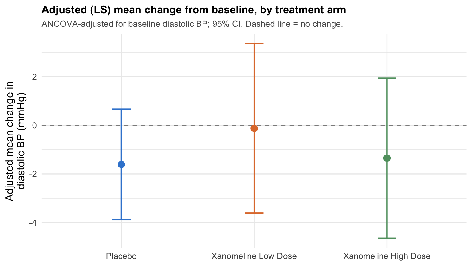
Here is where we are headed — the adjusted mean change from baseline in each arm, with its 95% CI, computed from the ANCOVA we build below:

Point-and-interval plot of the adjusted (least-squares) mean change from baseline in diastolic blood pressure at Week 24 for each treatment arm, with 95 percent confidence intervals. Placebo (azure) sits at about minus 1.6 mmHg, Xanomeline Low Dose (orange) at about minus 0.1 mmHg, and Xanomeline High Dose (green) at about minus 1.4 mmHg. A dashed horizontal line marks zero change. All three intervals span zero and overlap heavily, showing no clear treatment effect on this endpoint.

All three intervals straddle the dashed zero line and overlap heavily: on this endpoint the data show no treatment effect. That is a real result too, and by the end of this lesson you will have produced it as a formal ANCOVA table — and, just as important, be able to read whether a CI clears zero. If “ADaM”, “BDS”, “change from baseline”, or “treatment arm” are new, start with Create ADSL in R with admiral, which builds the subject-level dataset the population flags come from.

What an efficacy (ANCOVA) table shows

An efficacy table for a continuous endpoint has a fixed anatomy. It is the visible summary of one linear model — CHG ~ arm + baseline — read one arm per column:

Part	What it is	In this lesson
Endpoint	The continuous response, usually change from baseline (`CHG`)	Change in diastolic blood pressure at Week 24
Adjustment	The covariate(s) the model conditions on	Baseline value (`BASE`)
Columns	The treatment arms; the first is the reference	Placebo (ref) · Xanomeline Low · Xanomeline High
n	Subjects contributing to the model in that arm	Per-arm analyzed count
Adjusted (LS) mean	The arm’s mean change at the common mean baseline	e.g. Placebo −1.6 mmHg
Difference in LS means	Active arm minus the reference	e.g. Low − Placebo
95% CI	The interval around that difference	Excludes 0 ⇒ significant
p-value	Test that the difference is 0 (unadjusted for multiplicity)	e.g. 0.48

Three conventions decide whether the table is right:

The endpoint is the change, and baseline is a covariate — not the outcome. You model CHG (or AVAL with baseline adjustment), and BASE enters on the right-hand side as an adjustment term. Analysing change and adjusting for baseline is the standard ICH E9 approach: it removes the part of the outcome explained by where a subject started, so the treatment comparison is fair.
The means are adjusted, not raw. An arm’s cell is its least-squares (LS) mean — also called the estimated marginal mean — the model’s estimate of that arm’s mean change if all arms shared the same average baseline. When baseline differs across arms (it usually does, a little), the LS mean and the raw mean differ. Reporting the raw mean instead is a common mistake.
The comparison is against a fixed reference. One arm — here placebo — is the reference, and every difference is that active arm minus the reference. A 95% CI on the difference that excludes 0 is a statistically significant adjusted treatment effect; a CI that includes 0 is not.

The data

We use the ADVS (Analysis Data Vital Signs) dataset shipped in pharmaverseadam — the synthetic, license-free CDISC (Clinical Data Interchange Standards Consortium) pilot study comparing placebo against two doses of Xanomeline. ADVS is a BDS (Basic Data Structure) ADaM: one row per subject per parameter per visit, already carrying the analysis value AVAL, the baseline BASE, and the change from baseline CHG — so no derivation is needed here.

Our endpoint is the change from baseline in diastolic blood pressure (PARAMCD == "DIABP", in mmHg) at Week 24, the end of the double-blind treatment period. Diastolic blood pressure is a continuous clinical measure that stands in for the trial’s efficacy endpoint; in a real Alzheimer’s study the primary endpoint would be a cognitive score, but the ANCOVA table is built the identical way for any continuous change-from-baseline endpoint.

Three filters set up the analysis population. We keep the analysis records for the endpoint (PARAMCD, AVISIT, and — because vital signs are measured in several body positions — the supine reading ATPT == "AFTER LYING DOWN FOR 5 MINUTES", so there is exactly one row per subject); the analysis flag ANL01FL == "Y" (the record chosen for analysis); and the safety population SAFFL == "Y". Efficacy analyses are conventionally run on the intent-to-treat (ITT) or full-analysis population; this pilot ADaM ships only the safety flag, so we use it and note the distinction.

library(dplyr, warn.conflicts = FALSE)
library(pharmaverseadam)

arm_levels <- c("Placebo", "Xanomeline Low Dose", "Xanomeline High Dose")

# ADVS (BDS) — one row per subject per visit; keep the Week 24 diastolic-BP
# change-from-baseline analysis record, supine, for the safety population.
anl <- pharmaverseadam::advs %>%
  filter(
    PARAMCD  == "DIABP",
    AVISIT   == "Week 24",
    ATPT     == "AFTER LYING DOWN FOR 5 MINUTES",
    ANL01FL  == "Y",
    SAFFL    == "Y",
    !is.na(CHG), !is.na(BASE)
  ) %>%
  mutate(TRT01A = factor(TRT01A, levels = arm_levels))

anl %>%
  select(USUBJID, TRT01A, PARAM, AVISIT, BASE, AVAL, CHG) %>%
  head(5)

# A tibble: 5 × 7
  USUBJID     TRT01A               PARAM                AVISIT  BASE  AVAL   CHG
  <chr>       <fct>                <chr>                <chr>  <dbl> <dbl> <dbl>
1 01-701-1015 Placebo              Diastolic Blood Pre… Week …    56    63     7
2 01-701-1028 Xanomeline High Dose Diastolic Blood Pre… Week …    85    73   -12
3 01-701-1034 Xanomeline High Dose Diastolic Blood Pre… Week …    60    81    21
4 01-701-1097 Xanomeline Low Dose  Diastolic Blood Pre… Week …    72    83    11
5 01-701-1118 Placebo              Diastolic Blood Pre… Week …    84    76    -8

Making TRT01A a factor with placebo first does two jobs: it fixes the column order of the table (placebo, then ascending dose), and — because ANCOVA takes the first factor level as the reference — it makes placebo the comparator. Look at the raw picture before modelling:

anl %>%
  group_by(TRT01A) %>%
  summarise(
    n         = n(),
    mean_base = round(mean(BASE), 1),   # average baseline diastolic BP
    mean_chg  = round(mean(CHG), 2),    # raw mean change from baseline
    .groups   = "drop"
  )

# A tibble: 3 × 4
  TRT01A                   n mean_base mean_chg
  <fct>                <int>     <dbl>    <dbl>
1 Placebo                 59      73.9    -1.05
2 Xanomeline Low Dose     25      76.6    -0.8 
3 Xanomeline High Dose    28      76.4    -1.93

Two things to notice. The arms have 59, 25, and 28 analyzable subjects at Week 24 (the active arms are smaller — dropout thins the later visits). And the average baseline differs across arms (placebo starts a little lower), which is exactly why we adjust: the ANCOVA will report each arm’s change at the common mean baseline, so that starting difference does not leak into the treatment comparison.

Build the ANCOVA efficacy table

The tern layout-creating function for this is summarize_ancova(). You read the layout top-to-bottom as a recipe: start a table, split the columns by treatment arm naming the reference, add the column counts, then call summarize_ancova() with the endpoint (vars), the model’s arm and covariates, and the confidence level. Nothing is computed until build_table() applies the layout to the data — at which point tern fits lm(CHG ~ TRT01A + BASE), extracts the LS means with emmeans, and formats the rows.

library(rtables)
library(tern)

lyt <- basic_table(
    title     = "Table 14-2.01",
    subtitles = "ANCOVA of Change from Baseline in Diastolic BP at Week 24 (Safety Population)"
  ) %>%
  split_cols_by("TRT01A", ref_group = "Placebo") %>%   # placebo is the reference column
  add_colcounts() %>%                                  # the (N=xx) header row
  summarize_ancova(
    vars       = "CHG",
    variables  = list(arm = "TRT01A", covariates = "BASE"),  # CHG ~ TRT01A + BASE
    conf_level = 0.95,
    var_labels = "Change from Baseline (adjusted for baseline)"
  )

build_table(lyt, df = anl)

Table 14-2.01
ANCOVA of Change from Baseline in Diastolic BP at Week 24 (Safety Population)

———————————————————————————————————————————————————————————————————————————————————————————————————
                                               Placebo   Xanomeline Low Dose   Xanomeline High Dose
                                               (N=59)          (N=25)                 (N=28)       
———————————————————————————————————————————————————————————————————————————————————————————————————
Change from Baseline (adjusted for baseline)                                                       
  n                                              59              25                     28         
  Adjusted Mean                                 -1.61           -0.13                 -1.35        
  Difference in Adjusted Means                                  1.48                   0.26        
    95% CI                                                  (-2.69, 5.66)         (-3.75, 4.27)    
    p-value                                                    0.4823                 0.8983

The two arguments that define the analysis are ref_group = "Placebo" (in split_cols_by()) and variables = list(arm = "TRT01A", covariates = "BASE"). The arm is the treatment variable whose adjusted means we compare; covariates is the adjustment set — here just baseline, but you would add stratification factors (c("BASE", "STRATA1")) exactly the same way. conf_level = 0.95 sets the CI.

Read the output

Walk down the table the way a reviewer does:

n — 59 placebo, 25 low-dose, 28 high-dose subjects entered the model.
Adjusted Mean — the LS mean change from baseline, at the common mean baseline: about −1.6 mmHg on placebo, −0.1 on low dose, and −1.4 on high dose. These are the model’s fair per-arm estimates. Compare them with the raw means from the summary above — they differ slightly because baseline differed across arms; the LS means are the raw means after removing that baseline difference.
Difference in Adjusted Means — each active arm minus placebo: +1.5 mmHg for low dose and +0.3 mmHg for high dose. Positive here means the arm’s diastolic BP fell less than placebo’s.
95% CI — the low-dose difference is roughly (−2.7, 5.7) and the high-dose difference (−3.8, 4.3). Both intervals comfortably include 0.
p-value — 0.48 and 0.90, both far above 0.05.

The reading is unambiguous: adjusting for baseline, neither Xanomeline dose changes diastolic blood pressure differently from placebo — every CI spans zero and every p is large. When a 95% CI on the difference excludes 0 (equivalently p < 0.05), you have a statistically significant adjusted treatment effect; here you do not. A null result, cleanly reported, is exactly what this table exists to show, and its shape is identical to the one you would present for a positive trial — only the numbers change.

Note

The p-values tern reports are the unadjusted pairwise tests from the model. When a study has more than one active arm against a common control, the analysis plan may call for a multiplicity adjustment (Dunnett, Bonferroni, a gatekeeping procedure) so the family-wise error rate is controlled — the pre-specified statistical analysis plan decides which. That adjustment is layered on top of the same LS-means model.

When ANCOVA is not enough: a note on MMRM

The table above analyzes one visit (Week 24) and drops subjects who did not reach it — a complete-case ANCOVA. Modern longitudinal trials more often use a mixed model for repeated measures (MMRM): it models all post-baseline visits at once, uses every subject’s available data (so a subject who missed Week 24 but attended Week 20 still contributes), and handles the within-subject correlation across visits. MMRM is the primary-analysis default in many recent submissions because it makes weaker missing-data assumptions than single-visit ANCOVA or last-observation-carried-forward. The reporting table looks much the same — LS means per arm, a difference, a CI, a p — which is why ANCOVA is the right place to learn the pattern first. MMRM is a topic for its own lesson; the model is fitted with the mmrm package and tabulated with tern.mmrm.

🟢 With an AI agent

Ask Prova “how do I add a stratification factor to my tern summarize_ancova efficacy table, and how does that change the LS means?” — it answers grounded in this pillar’s lessons, with runnable code you can try on the example pharmaverse data. The runtime is the judge. Ask Prova →

Common issues

You reported the raw means, not the LS means. A group_by(arm) |> summarise(mean(CHG)) gives the unadjusted mean change; the efficacy table reports the least-squares mean from the ANCOVA — the mean adjusted to the common baseline. They differ whenever baseline is imbalanced across arms (almost always, a little). summarize_ancova() returns the LS mean (lsmean); do not overwrite it with a raw aggregate().

Baseline is on the wrong side of the model. The endpoint is the change (CHG), and the baseline (BASE) is a covariate — it belongs in covariates, on the right of the formula, never as the response. If you accidentally model BASE as the outcome (or analyze AVAL without adjusting for BASE at all), the table answers the wrong question. Model CHG ~ arm + BASE.

The wrong arm is the reference. ANCOVA takes the first factor level of the arm variable as the reference, and split_cols_by(..., ref_group = "Placebo") makes that explicit. If placebo is not first (e.g. the arms fell alphabetical, so “Xanomeline High Dose” leads), every “difference” is computed against the wrong comparator and flips sign. Set the factor levels with placebo first and pass ref_group.

More than one row per subject sneaks into the model. ANCOVA expects one analysis record per subject. Vital signs are measured in several body positions and at several timepoints, so without pinning the parameter, visit, position, and analysis flag (PARAMCD, AVISIT, ATPT, ANL01FL == "Y") you can hand the model three rows per subject and silently inflate n. Filter to a single analysis record first, and check n() per arm before modelling.

Frequently asked questions

What is an efficacy table in a clinical trial?

It is the table that reports the trial’s primary (or key secondary) endpoint result — the formal answer to did the treatment work? For a continuous endpoint it is an ANCOVA (analysis of covariance) of the change from baseline: per treatment arm it shows the number of subjects and the adjusted (least-squares) mean change, then, for each active arm versus the reference, the difference in adjusted means with a 95% CI and p-value, adjusting for the baseline value. It sits in section 14.2 of a Clinical Study Report, whose structure follows the ICH E3 guideline.

How do I build an ANCOVA table in R with rtables and tern?

Use summarize_ancova(): basic_table() |> split_cols_by("TRT01A", ref_group = "Placebo") |> add_colcounts() |> summarize_ancova(vars = "CHG", variables = list(arm = "TRT01A", covariates = "BASE"), conf_level = 0.95), then apply it with build_table(df = anl). tern fits lm(CHG ~ TRT01A + BASE), extracts the least-squares means with emmeans, and lays out n, the adjusted mean, the difference, the CI, and the p-value. The full build is worked through above on public pharmaverse data.

What are LS means (least-squares means) and how do they differ from raw means?

A least-squares mean (also called an estimated marginal mean) is a model-based estimate of an arm’s mean at a common value of the covariates — here, the mean change from baseline if every arm had the same average baseline. A raw mean just averages the observed values in the arm. They coincide only when the covariate is perfectly balanced across arms; when baseline differs (as it usually does), the LS mean is the fair, adjusted estimate and the raw mean is not. The efficacy table always reports the LS mean.

Why adjust for baseline in an efficacy analysis?

Because part of a subject’s outcome is explained by where they started. Adjusting for the baseline value (as a covariate) removes that variability, which increases the precision of the treatment estimate and protects against a chance baseline imbalance being read as a treatment effect. Analysing change from baseline and including baseline as a covariate is the standard approach recommended in ICH E9 and the EMA/FDA baseline-covariate guidance.

How do I read the adjusted mean difference and its confidence interval?

The difference in adjusted means is the active arm’s LS mean minus the reference arm’s LS mean — the estimated treatment effect on the endpoint, in the endpoint’s units. Its 95% CI is the range of effects compatible with the data: if the interval excludes 0 the effect is statistically significant (equivalently p < 0.05); if it includes 0, as in this lesson’s table, there is no significant difference from the reference. Always read the CI, not just the p-value — its width tells you how precise the estimate is.

ANCOVA or MMRM for the efficacy analysis?

ANCOVA analyzes a single timepoint (e.g. the end-of-treatment visit) as change from baseline adjusted for baseline — simple, and what this lesson builds. MMRM (mixed model for repeated measures) analyzes all post-baseline visits jointly, keeps subjects with partial follow-up, and models the within-subject correlation, so it makes weaker missing-data assumptions and is the primary-analysis default in many recent trials. The reporting table looks the same (LS means, a difference, a CI, a p); the model is fitted with the mmrm package and tabulated with tern.mmrm. Learn ANCOVA first — the pattern transfers directly.

Test your understanding

Your turn: add the raw mean and compare

Using the anl object from this lesson, build the same ANCOVA table but add the raw arithmetic mean of CHG as an extra statistic, so you can see the adjusted (LS) mean and the raw mean side by side. Which arm’s LS mean moves furthest from its raw mean, and why?

Hint

summarize_ancova()’s .stats argument controls which statistics appear; the default is c("n", "lsmean", "lsmean_diff", "lsmean_diff_ci", "pval"). It does not offer a raw mean, so compute it separately with group_by(TRT01A) |> summarise(raw = mean(CHG)) and read it next to the table. The LS mean will differ most from the raw mean in the arm whose baseline is furthest from the overall mean baseline — that is the arm the baseline adjustment moves most.

Solution

library(dplyr)
library(rtables)
library(tern)

# the LS (adjusted) means — from the ANCOVA
lyt <- basic_table() %>%
  split_cols_by("TRT01A", ref_group = "Placebo") %>%
  add_colcounts() %>%
  summarize_ancova(
    vars = "CHG",
    variables = list(arm = "TRT01A", covariates = "BASE"),
    conf_level = 0.95,
    var_labels = "Change from Baseline (adjusted)"
  )
build_table(lyt, df = anl)

# the RAW means and mean baselines — for comparison
anl %>%
  group_by(TRT01A) %>%
  summarise(n = n(), mean_base = round(mean(BASE), 1),
            raw_mean_chg = round(mean(CHG), 2), .groups = "drop")

The adjusted (LS) mean and the raw mean differ because the arms’ average baselines differ. The arm whose mean baseline sits furthest from the overall average is shifted most by the adjustment — that shift is precisely what ANCOVA does, and why the efficacy table reports the LS mean rather than the raw mean.

Quick check: in an efficacy ANCOVA table, what does the “Adjusted Mean” for an arm represent?

A. The raw arithmetic mean of change from baseline in that arm B. The arm’s mean change from baseline estimated at the common mean baseline (the LS mean) C. The difference between that arm and placebo

Show answer

B. The “Adjusted Mean” is the least-squares (LS) mean — the model’s estimate of the arm’s mean change if all arms shared the same average baseline. A is the raw mean, which ignores the baseline adjustment and differs whenever baseline is imbalanced; C is the separate “Difference in Adjusted Means” row, the LS mean of the arm minus the LS mean of the reference.

Conclusion

The efficacy table is the primary-endpoint read-out of a Clinical Study Report, and for a continuous endpoint it comes down to one linear model: change from baseline, adjusted for baseline, compared across arms. With rtables and tern that model is one layout call — summarize_ancova(vars = "CHG", variables = list(arm = "TRT01A", covariates = "BASE")) inside a split_cols_by("TRT01A", ref_group = "Placebo") — and the output is the standard table: n and the adjusted LS mean per arm, then the difference in LS means with its 95% CI and p-value against the reference. Read the CI first: excludes zero and the effect is significant; includes zero, as here, and it is not. Get three things right — model the change with baseline as a covariate, report the LS mean not the raw mean, and fix the reference arm — and your efficacy table answers the trial’s central question correctly, whichever way the numbers fall.

Note

This lesson is reproducible: every result on this page was produced by the code shown — copy any block and run it to reproduce them. The runtime is the judge.

Reuse

CC BY-NC-SA 4.0

Citation

BibTeX citation:

@online{2026,
  author = {},
  title = {The {Efficacy} {Table} in {R:} {ANCOVA} and {LS} {Means} with
    Rtables and Tern},
  date = {2026-07-01},
  url = {https://www.datanovia.com/learn/pharma-clinical/04-tlf-generation/efficacy-table-tern},
  langid = {en}
}

For attribution, please cite this work as:

“The Efficacy Table in R: ANCOVA and LS Means with Rtables and Tern.” 2026. July 1. https://www.datanovia.com/learn/pharma-clinical/04-tlf-generation/efficacy-table-tern.