The Analysis Results Dataset (ARD) in R: Results as Data with cards and cardx

Compute every result once as a tidy, one-row-per-statistic dataset — the CDISC Analysis Results Standard — with the pharmaverse cards and cardx packages, then feed the same object to a table, a filter, or a plot, so the computation of a result is finally separated from its display

A complete, runnable tutorial for the Analysis Results Dataset (ARD) — the tidy, one-row-per-result data structure that the CDISC Analysis Results Standard puts at the centre of clinical reporting. Learn what an ARD is and why “results as data” matters (it decouples the computation of a statistic from how it is displayed), then build one with the pharmaverse cards and cardx packages: ard_continuous() for summary statistics, ard_categorical() for counts and percentages, cardx::ard_stats_t_test() for a test result as data, and bind_ard() to stack them. Finally connect the ARD to a display with gtsummary::tbl_ard_summary(), and — because the ARD is just a tibble — filter it and plot a single number with ggplot2. Runs on public pharmaverseadam ADSL data, so every line executes.

TipKey takeaways

• An ARD (Analysis Results Dataset) is your results stored as data — one row per statistic (a mean, a count, a percentage, a p-value), each tagged with the variable it describes, the group it belongs to, and how it should be formatted. It is the data structure at the heart of the CDISC Analysis Results Standard (ARS).
• It decouples computing a result from displaying it. You calculate every number once into a tidy dataset; a table, a listing, or a figure is then just a view of that dataset — not a fresh calculation. Compute once, display many ways.
• cards builds descriptive ARDs. ard_continuous() gives you N, mean, SD, median, and quartiles by group; ard_categorical() gives you n, N, and percentages.
• cardx turns tests into ARDs. ard_stats_t_test() runs a t-test and returns the estimate, statistic, degrees of freedom, CI, and p-value as rows — a test result you can filter, not re-run.
• The ARD is just a tibble, so a table, a filter, and a plot all come from it. Feed it to gtsummary::tbl_ard_summary() for a display table, subset it with base [ to pull one number, or hand the same rows to ggplot2.

Introduction

You computed the demographic table, the adverse-event table, and the efficacy result — three times, on three different machines, in three different scripts. The mean age lives inside a gtsummary object; the event counts live inside an rtables layout; the p-value lives in the console output of a t.test(). Ask a simple cross-cutting question — what was the mean age in the placebo arm? — and you are digging through formatted table cells to recover a number that was, at some point, a plain numeric value.

The Analysis Results Dataset (ARD) fixes this by turning that question on its head: what if every result were just… data? An ARD is a tidy dataset with one row per computed statistic. The mean age in the placebo arm is a row. The percentage of female subjects on the high dose is a row. The treatment-comparison p-value is a row. Each row carries not just the number but its context — which variable, which group, which statistic, and how to format it. This is what “results as data” means: a computed result is stored as a record in a dataset, not baked into a formatted table cell.

This idea is now a formal CDISC standard. CDISC (Clinical Data Interchange Standards Consortium) — the body behind the clinical-data models the industry submits to regulators — publishes the Analysis Results Standard (ARS), which specifies the ARD as the machine-readable structure that sits between the analysis datasets and the final TLF (tables, listings, and figures). Just as ADaM (Analysis Data Model) standardised the analysis-ready data, ARS standardises the analysis results. In R, the pharmaverse packages cards and cardx build ARDs and connect them to displays.

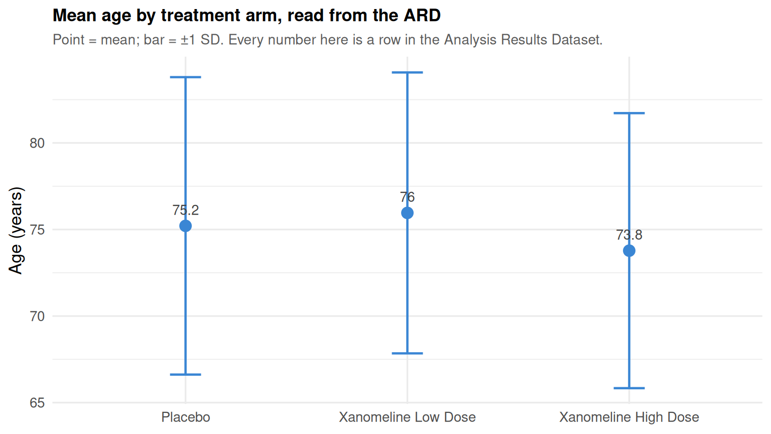
Here is the payoff, up front — a figure drawn directly from an ARD, not from a re-run analysis:

The mean and the standard deviation behind each point were not recomputed for the plot — they were filtered out of the ARD we build below. That is the whole lesson: compute the results once into a dataset, then table them, filter them, or plot them from the same object.

What an ARD is (and why “results as data”)

A traditional reporting script computes and formats in one breath: it runs a summary and immediately renders a table. The number and its presentation are welded together, so the number is hard to reuse and the table is hard to change without re-running the analysis.

An ARD breaks that weld into two clean steps:

1. Compute — produce a tidy dataset of results, one row per statistic, with full context (variable, group, statistic name, value, format).
2. Display — render any view (a gtsummary table, an rtables layout, a figure) as a transformation of that dataset.

The benefits are the reasons CDISC standardised it: a result computed once can feed many outputs (so the mean in your table and the mean in your figure are provably the same number); results become traceable and machine-readable (an ARD row records exactly what was computed and how); and a display change never risks changing a value, because the value already exists as data. The Analysis Results Standard formalises this so results can move between tools and sponsors the way ADaM datasets already do.

The rest of this lesson builds an ARD from a real analysis dataset and connects it to a display.

The data

We use ADSL (the subject-level analysis dataset — one row per subject, carrying treatment, demographics, and population flags) shipped in pharmaverseadam, the synthetic, license-free CDISC pilot study comparing placebo against two doses of Xanomeline. It arrives as a tibble, so the first move is as.data.frame() — the cards functions and base-R subsetting we use throughout expect a plain data frame. We also keep the three real treatment arms (dropping the screen-failure rows, who were never randomised) and fix their order with a factor, so placebo leads every table and figure.

library(cards)

# ADSL is a tibble -> make it a plain data.frame first.
arms <- c("Placebo", "Xanomeline Low Dose", "Xanomeline High Dose")
adsl <- as.data.frame(pharmaverseadam::adsl)
adsl <- adsl[adsl$TRT01A %in% arms, ]           # keep the randomised arms
adsl$TRT01A <- factor(adsl$TRT01A, levels = arms)

adsl[1:5, c("USUBJID", "TRT01A", "AGE", "SEX", "RACE")]

      USUBJID               TRT01A AGE SEX  RACE
1 01-701-1015              Placebo  63   F WHITE
2 01-701-1023              Placebo  64   M WHITE
3 01-701-1028 Xanomeline High Dose  71   M WHITE
4 01-701-1033  Xanomeline Low Dose  74   M WHITE
5 01-701-1034 Xanomeline High Dose  77   F WHITE

TRT01A is the actual treatment arm; AGE, SEX, and RACE are the demographics we will summarise. That is all the ARD needs.

Build a continuous ARD with ard_continuous()

The first ARD summarises a continuous variable. Point ard_continuous() at the data, name the grouping variable with by, and name the variable(s) to summarise. It returns a card tibble — the ARD — with the standard battery of statistics (N, mean, SD, median, quartiles, min, max) for each group.

library(cards)

arms <- c("Placebo", "Xanomeline Low Dose", "Xanomeline High Dose")
adsl <- as.data.frame(pharmaverseadam::adsl)
adsl <- adsl[adsl$TRT01A %in% arms, ]
adsl$TRT01A <- factor(adsl$TRT01A, levels = arms)

ard_age <- ard_continuous(adsl, by = TRT01A, variables = AGE)

# show the Placebo arm's statistics (the first block of rows).
# group1_level is a list-column, so unlist() it before the comparison.
ard_age[unlist(ard_age$group1_level) == "Placebo",
        c("group1_level", "variable", "stat_name", "stat_label", "stat")]

  group1_level variable stat_name stat_label   stat
1      Placebo      AGE         N          N     86
2      Placebo      AGE      mean       Mean 75.209
3      Placebo      AGE        sd         SD   8.59
4      Placebo      AGE    median     Median     76
5      Placebo      AGE       p25         Q1     69
6      Placebo      AGE       p75         Q3     82
7      Placebo      AGE       min        Min     52
8      Placebo      AGE       max        Max     89

Read one row: for the placebo arm, the mean of AGE is 75.2. Every summary number the demographic table would ever show is now a row you can point to. The card tibble carries more columns than we printed — this is the anatomy of an ARD:

Column	What it holds	Example
group1	The grouping variable	TRT01A
group1_level	The grouping value for this row	Placebo
variable	The variable being summarised	AGE
stat_name	Which statistic this row is	mean, sd, median, p25, N
stat_label	A human-readable label for it	Mean, SD, Median
stat	The computed value	75.2093
context	The kind of analysis that produced it	continuous
fmt_fun	How to format the value for display	round to 1 decimal
warning / error	Anything the computation emitted	usually empty

Two columns carry the “results as data” idea. stat is the number itself, stored as data rather than as a formatted string; fmt_fun records how to display it separately from the value — so rounding is a display decision applied later, not baked into the result. That separation is the entire point of the standard.

Build a categorical ARD with ard_categorical()

A categorical variable needs counts and percentages instead of a mean. ard_categorical() has the same shape of call and returns, for each level of the variable, the count n, the denominator N, and the proportion p.

library(cards)

arms <- c("Placebo", "Xanomeline Low Dose", "Xanomeline High Dose")
adsl <- as.data.frame(pharmaverseadam::adsl)
adsl <- adsl[adsl$TRT01A %in% arms, ]
adsl$TRT01A <- factor(adsl$TRT01A, levels = arms)

ard_sex <- ard_categorical(adsl, by = TRT01A, variables = SEX)

ard_sex[unlist(ard_sex$group1_level) == "Placebo",
        c("group1_level", "variable", "variable_level", "stat_name", "stat")]

  group1_level variable variable_level stat_name  stat
1      Placebo      SEX              F         n    53
2      Placebo      SEX              F         N    86
3      Placebo      SEX              F         p 0.616
4      Placebo      SEX              M         n    33
5      Placebo      SEX              M         N    86
6      Placebo      SEX              M         p 0.384

For the placebo arm there are 53 female subjects (n) out of 86 (N), a proportion of 0.616 (p) — the 61.6% a demographic table would print. Note the extra variable_level column: a categorical ARD needs a row per category, so it records which level (F or M) each n/N/p belongs to. The continuous ARD had no such column because a mean has no sub-levels.

Turn a test into an ARD with cardx::ard_stats_t_test()

Descriptive statistics are one kind of result; an inferential test is another. The cardx package extends cards to statistical tests — and it returns the test as an ARD, so a p-value becomes a row exactly like a mean does.

ard_stats_t_test() runs a two-sample t-test. It compares exactly two groups, so the by variable must have exactly two levels — we subset to placebo versus the high dose first.

library(cards)
library(cardx)

arms <- c("Placebo", "Xanomeline Low Dose", "Xanomeline High Dose")
adsl <- as.data.frame(pharmaverseadam::adsl)
adsl <- adsl[adsl$TRT01A %in% arms, ]
adsl$TRT01A <- factor(adsl$TRT01A, levels = arms)

# t-test needs exactly two groups: Placebo vs High Dose
two <- adsl[adsl$TRT01A %in% c("Placebo", "Xanomeline High Dose"), ]
two$TRT01A <- factor(two$TRT01A)

ard_tt <- ard_stats_t_test(data = two, by = TRT01A, variable = AGE)

ard_tt[ard_tt$stat_name %in%
         c("estimate", "statistic", "parameter", "p.value", "conf.low", "conf.high"),
       c("variable", "stat_name", "stat_label", "stat")]

  variable stat_name stat_label    stat
1      AGE  estimate  Mean Dif…   1.432
2      AGE statistic  t Statis…   1.087
3      AGE   p.value    p-value   0.279
4      AGE parameter  Degrees … 154.432
5      AGE  conf.low  CI Lower…   -1.17
6      AGE conf.high  CI Upper…   4.033

Every piece of a t-test is now a labelled row: the estimate is the mean age difference (about 1.4 years, placebo minus high dose); statistic is the t value (1.09); parameter is the degrees of freedom (Welch’s, ≈154); conf.low/conf.high are the 95% CI (−1.2 to 4.0); and p.value is 0.28. The interval spans zero and the p-value is far above 0.05 — the arms are well-matched on age, which is what you want in a randomised trial. The result of the test is now queryable data, not a block of console text you have to scrape.

Stack ARDs with bind_ard()

Real reporting needs many results together — several variables, both descriptive and inferential. bind_ard() stacks any number of ARDs into one, because they all share the same column structure. That single stacked ARD is what a display consumes.

library(cards)

arms <- c("Placebo", "Xanomeline Low Dose", "Xanomeline High Dose")
adsl <- as.data.frame(pharmaverseadam::adsl)
adsl <- adsl[adsl$TRT01A %in% arms, ]
adsl$TRT01A <- factor(adsl$TRT01A, levels = arms)

ard_age <- ard_continuous(adsl, by = TRT01A, variables = AGE)
ard_sex <- ard_categorical(adsl, by = TRT01A, variables = SEX)

ard_demo <- bind_ard(ard_age, ard_sex)

# how many result rows, and for which variables
table(ard_demo$variable)

AGE SEX 
 24  18 

ard_demo now holds every age statistic and every sex count/percentage for all three arms in one tidy object — the machine-readable results behind a demographic table, ready to display.

Connect the ARD to a display: gtsummary::tbl_ard_summary()

The ARD is the computation; a table is one display of it. gtsummary::tbl_ard_summary() takes a pre-computed ARD and lays it out as a publication-ready summary table — it does no statistics of its own, it only arranges the numbers the ARD already holds.

library(cards)
library(gtsummary)

arms <- c("Placebo", "Xanomeline Low Dose", "Xanomeline High Dose")
adsl <- as.data.frame(pharmaverseadam::adsl)
adsl <- adsl[adsl$TRT01A %in% arms, ]
adsl$TRT01A <- factor(adsl$TRT01A, levels = arms)

ard_demo <- bind_ard(
  ard_continuous(adsl, by = TRT01A, variables = AGE),
  ard_categorical(adsl, by = TRT01A, variables = SEX)
)

tbl_ard_summary(ard_demo, by = "TRT01A")

Table 1

Characteristic	Placebo1	Xanomeline Low Dose1	Xanomeline High Dose1
AGE	76.0 (69.0, 82.0)	78.0 (71.0, 82.0)	75.5 (70.0, 79.0)
SEX
F	53 (61.6%)	55 (57.3%)	35 (48.6%)
M	33 (38.4%)	41 (42.7%)	37 (51.4%)
1 Median (Q1, Q3); n (%)

That is the demographic table — age as median (Q1, Q3), sex as n (%) — and not a single statistic was recomputed to make it. Every cell was read from ard_demo. Change the display (round differently, reorder rows, switch to an rtables layout) and the underlying results never move.

This is also the cleanest way to see cards versus gtsummary. The ordinary gtsummary::tbl_summary() computes and displays in one call — convenient, but the numbers live inside the table object. tbl_ard_summary() displays an ARD you built separately, so the results exist as data first and the table is just a view. Use tbl_summary() for a quick one-off; build an ARD when the same results must feed several outputs, be traced, or follow the CDISC standard.

Results as data: filter and plot from the ARD

Because the ARD is a plain tibble, you do not need a special function to reuse a result — base R is enough. Filtering the ARD to one statistic gives you a clean data frame you can print, report, or plot. This is exactly how the hero figure at the top was made: pull the mean rows, pull the sd rows, and hand them to ggplot2.

library(cards)
library(ggplot2)

arms <- c("Placebo", "Xanomeline Low Dose", "Xanomeline High Dose")
adsl <- as.data.frame(pharmaverseadam::adsl)
adsl <- adsl[adsl$TRT01A %in% arms, ]
adsl$TRT01A <- factor(adsl$TRT01A, levels = arms)

ard_sex <- ard_categorical(adsl, by = TRT01A, variables = SEX)

# filter the ARD to the % of female subjects, per arm (base R)
female_pct <- ard_sex[ard_sex$stat_name == "p" & ard_sex$variable_level == "F", ]
pct <- data.frame(
  arm = factor(unlist(female_pct$group1_level), levels = arms),
  pct = 100 * as.numeric(female_pct$stat)
)

ggplot(pct, aes(x = arm, y = pct)) +
  geom_col(fill = "#3a86d4", width = 0.6) +
  geom_text(aes(label = paste0(round(pct), "%")), vjust = -0.4, size = 3.8, colour = "grey25") +
  labs(x = NULL, y = "Female subjects (%)",
       title = "Percentage female by arm, drawn straight from the ARD") +
  theme_minimal(base_size = 13) +
  theme(plot.title = element_text(face = "bold", size = 13))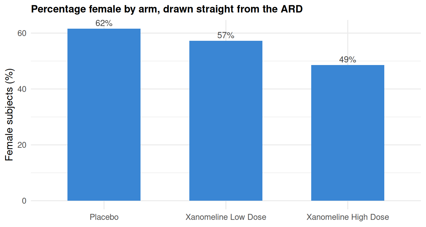

Nothing here recomputes a percentage: 100 * as.numeric(female_pct$stat) reads the proportion that already sits in the ARD. The table above and this figure now report the same numbers by construction — which is the guarantee the ARD exists to give.

🟢 With an AI agent

Ask Prova “how do I add a mean and SD row to my cards ARD and control how each statistic is formatted with the fmt_fun column?” — it answers grounded in this pillar’s lessons, with runnable cards/cardx code you can try on the example pharmaverse data. The runtime is the judge. Ask Prova →

Common issues

“no applicable method” or odd errors from ard_continuous() — you passed a tibble. pharmaverseadam::adsl is a tibble, and the tidiest fix is to convert it first: adsl <- as.data.frame(pharmaverseadam::adsl). Do this once at the top of every block; the base-R subsetting (adsl[...]) and the cards calls both behave on a plain data frame.

ard_stats_t_test() returns blank stats for three arms. A two-sample t-test compares exactly two groups, so the by variable must have exactly two levels. TRT01A has three arms (plus screen-failure rows if you did not drop them). cards does not raise a console error here — it captures the “grouping factor must have exactly 2 levels” message in the ARD’s error column and leaves stat empty. Subset to the two arms you want and re-factor so no empty level lingers: two <- adsl[adsl$TRT01A %in% c("Placebo", "Xanomeline High Dose"), ]; two$TRT01A <- factor(two$TRT01A).

You reached for shuffle_ard() — it is deprecated. Older tutorials pivot an ARD with shuffle_ard(), but it is deprecated in cards 0.8.0. To combine ARDs use bind_ard() (stacking), and to display one use gtsummary::tbl_ard_summary(); reshaping for a custom layout now lives in downstream display packages (tfrmt::shuffle_card()), not in cards.

A filter on group1_level (or variable_level) returns zero rows. The stat, group1_level, and variable_level columns of a card tibble are list-columns — and group1_level holds factors. Comparing a list-column with == (e.g. ard$group1_level == "Placebo") silently returns all FALSE, so the subset is empty. unlist() the column first so == compares values: ard[unlist(ard$group1_level) == "Placebo", ]. Same rule when you pull a number — subset the rows, then coerce the stat list-column: rows <- ard[unlist(ard$group1_level) == "Placebo" & ard$stat_name == "mean", ]; as.numeric(rows$stat).

Frequently asked questions

NoteWhat is an ARD (Analysis Results Dataset)?

An ARD is a tidy dataset in which each row is one computed result — a statistic such as a mean, a count, a percentage, or a p-value — tagged with the variable it describes, the group it belongs to, the statistic’s name, its value, and how to format it. It is the machine-readable structure the CDISC Analysis Results Standard places between the analysis datasets and the final tables and figures, so that results can be stored, traced, and reused as data.

NoteWhat does “results as data” actually mean?

It means storing a computed result as a record in a dataset instead of baking it into a formatted table cell. The number 75.2 for “mean age, placebo arm” becomes a row you can query, filter, and reuse — separate from any decision about how to round or lay it out. Because the computation is separated from the display, the same result can feed a table, a listing, and a figure and be provably identical in each.

Notecards vs gtsummary — which one do I use?

Use gtsummary’s tbl_summary() for a fast, one-call summary table when the numbers only need to appear in that one table. Use cards to build an ARD first — when the same results must feed several outputs, be traceable, or follow the CDISC standard — and then display it with tbl_ard_summary(). In short: tbl_summary() computes and displays together; cards + tbl_ard_summary() computes into a dataset first and displays second.

NoteWhy put results in a dataset at all?

Three reasons drove CDISC to standardise it. Consistency: a result computed once into an ARD can feed many outputs, so a table and a figure cannot silently disagree. Traceability: each ARD row records exactly what was computed, on which group, with what result — auditable and machine-readable. Separation of concerns: changing a display can never change a value, because the value already exists as data. Together these make reporting reproducible and portable across tools and sponsors.

NoteWhat is the difference between cards and cardx?

cards builds descriptive ARDs — summary statistics with ard_continuous() and counts/percentages with ard_categorical() — plus the utilities like bind_ard(). cardx (cards extra) extends it to statistical tests and models, returning them as ARDs too: ard_stats_t_test(), ANOVA, regression, and more. Descriptive summaries come from cards; tests come from cardx.

Test your understanding

ImportantYour turn: build a RACE ARD and pull one number

Using the adsl object from this lesson (the three randomised arms), build a categorical ARD for RACE, then read off — with base R, not by recomputing — the percentage of White subjects in the placebo arm.

TipHint

ard_categorical(adsl, by = TRT01A, variables = RACE) gives you n, N, and p per race level per arm. Filter the resulting ARD to the rows where stat_name == "p", unlist(variable_level) == "WHITE", and unlist(group1_level) == "Placebo" (unlist the list-columns so == compares values, not lists), then coerce the value: as.numeric(rows$stat) * 100.

TipSolution

library(cards)

arms <- c("Placebo", "Xanomeline Low Dose", "Xanomeline High Dose")
adsl <- as.data.frame(pharmaverseadam::adsl)
adsl <- adsl[adsl$TRT01A %in% arms, ]
adsl$TRT01A <- factor(adsl$TRT01A, levels = arms)

ard_race <- ard_categorical(adsl, by = TRT01A, variables = RACE)

rows <- ard_race[ard_race$stat_name == "p" &
                 unlist(ard_race$variable_level) == "WHITE" &
                 unlist(ard_race$group1_level) == "Placebo", ]
round(as.numeric(rows$stat) * 100, 1)   # % White in the placebo arm -> 90.7

The value is read straight from the ARD’s proportion (p) row — no table(), no re-tabulation. That is the point: once the result is data, reusing it is a filter.

NoteQuick check: what does one row of an ARD represent?

A. One subject in the study B. One computed statistic (e.g. the mean of AGE in the placebo arm) C. One formatted table cell, including its rounding and styling

TipShow answer

B. Each row of an Analysis Results Dataset is one computed statistic, tagged with its variable, group, name, value, and format. A describes the analysis data (ADSL is one row per subject); an ARD is one row per result. C is wrong because the value and its formatting are kept separate — the number lives in stat, the display rule lives in fmt_fun — which is exactly what lets one result feed many displays.

Conclusion

An ARD is your results turned into data: one row per statistic, each with the context needed to display it. That single shift — compute once into a dataset, display many ways — is what the CDISC Analysis Results Standard formalises, and what the pharmaverse cards and cardx packages give you in R. Build descriptive results with ard_continuous() and ard_categorical(), turn tests into results with cardx::ard_stats_t_test(), stack them with bind_ard(), and display the whole thing with gtsummary::tbl_ard_summary(). Because the ARD is just a tibble, the same results also feed a base-R filter or a ggplot2 figure — so your table, your listing, and your plot report provably the same numbers. Compute the result once; let every output be a view of it.

Note

This lesson is reproducible: every result on this page was produced by the code shown — copy any block and run it to reproduce them. The runtime is the judge.

Related lessons

• The rtables demographic table — the same demographic result built as a submission-grade display; an ARD is the tidy results layer that can feed it. · The efficacy table: ANCOVA and LS means — a modelled result (the kind cardx also turns into an ARD) laid out with rtables/tern. · Create ADSL in R with admiral — the subject-level analysis dataset that an ARD summarises.
• Where this fits: building ADaM with admiral (ADSL, ADVS, ADTTE) → producing the results — an ARD (you are here) is the tidy, standardised results layer — → generating the tables, listings, and figures (the demographic, adverse-event, and efficacy tables; the Kaplan-Meier figure) → packaging the submission.

Was this page helpful?

Prove you can do it. Master the whole Clinical Programming in R (pharmaverse) series — track your path, build projects, and earn a certificate.

Start free →

Go Pro — unlimited Prova on your own data and a verifiable certificate that proves the skill.

from $15/mo billed yearly

Go Pro →

✓ You're Pro — keep going. The runtime is the judge.

Get new R & Python lessons by email

Practical, reproducible, no spam. Unsubscribe anytime.

Double opt-in. We never share your email.

Share this pageXLinkedInRedditHN