Create ADSL in R with admiral: the Subject-Level Analysis Dataset

Derive a CDISC-conformant ADSL — treatment variables, populations, disposition, and age groups — from SDTM with admiral, the one-row-per-subject backbone every other ADaM dataset builds on

A complete, runnable tutorial for ADSL, the Subject-Level Analysis Dataset. Learn what ADSL is (one row per subject — the source of treatment variables, population flags, disposition, and demographics for every downstream ADaM and TLF), then build a conformant ADSL in R from SDTM source domains (DM, EX, DS) with admiral: derive_vars_merged() for treatment dates, derive_var_trtdurd() for treatment duration, derive_vars_cat() for age groups, and population flags such as SAFFL and RANDFL — on public pharmaverse data, so every line runs.

TipKey takeaways

• ADSL is the spine of every analysis. It holds one row per subject and is the single source of treatment variables, population flags, disposition, and demographics that every other ADaM dataset and every table, listing, and figure reads back from.
• You build it from SDTM, not from scratch. Subject attributes come from DM, treatment start/end dates from EX, and disposition (end of study, randomization) from DS — admiral merges them onto one subject-level frame.
• admiral derives it declaratively. derive_vars_merged() brings the right record from a source domain onto each subject, derive_var_trtdurd() computes treatment duration, and derive_vars_cat() builds analysis groupings such as AGEGR1 from a small lookup — no hand-rolled case_when() date logic.
• Population flags decide who is analyzed. SAFFL (safety: ever dosed) and RANDFL (randomized) are "Y"/"N" columns that downstream analyses filter on — get them right in ADSL and every count downstream is right.
• One row per subject is the contract. The final sanity check is that the number of rows equals the number of distinct USUBJID. If it does, ADSL is ready to merge into ADAE, ADTTE, ADLB, and the demographic table.

Introduction

Before a single demographic table, adverse-event summary, or Kaplan-Meier curve can be produced, someone has to build ADSL — the Subject-Level Analysis Dataset. ADSL is the first ADaM (Analysis Data Model) dataset you create and the one every other dataset depends on: it carries, for each subject exactly once, their treatment, their analysis populations, their disposition, and the demographic groupings that every downstream table will split by.

Get ADSL right and the rest of the deliverable falls into place, because every other ADaM dataset merges its key variables back from ADSL rather than re-deriving them. Get it wrong — a duplicated subject, a mis-set safety flag — and the error propagates into every count in the submission. This lesson builds a conformant ADSL in R with admiral, the pharmaverse package for ADaM derivation, working on public pharmaverse example data so every line runs as written. The build follows admiral’s official ADSL vignette, re-authored into a single guided walkthrough.

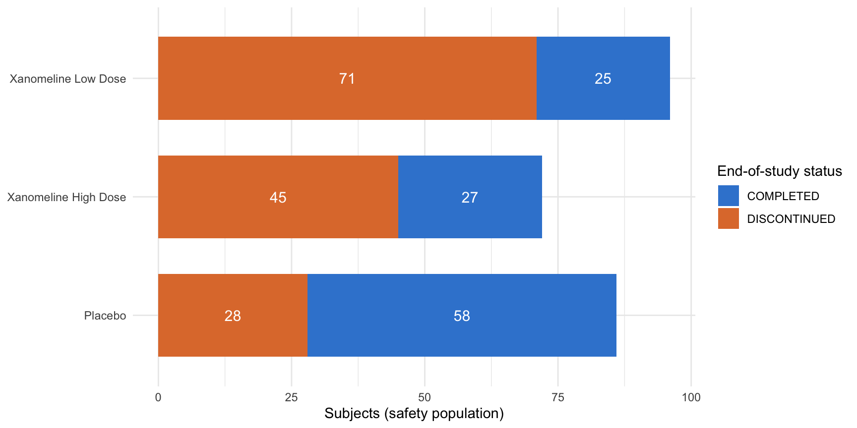
Here is where we are headed — disposition by treatment arm, computed straight from the ADSL we derive:

That figure reads off four ADSL columns — TRT01A, EOSSTT, SAFFL, and one row per subject. By the end of this lesson you will have derived all of them. If “ADaM”, “BDS”, or “SDTM” are new, start with the CDISC standards, which maps where ADSL sits. Coming from SAS? The SAS-to-R map explains why admiral plays the role of a validated derivation macro library.

What ADSL is

ADSL is the Subject-Level Analysis Dataset defined by the CDISC ADaM standard. Its structure is the simplest in all of ADaM and the reason everything else hangs off it: exactly one row per subject, keyed by USUBJID. There is no PARAMCD, no visit, no repeat — one subject, one row, many columns.

Every other ADaM dataset (ADAE, ADTTE, ADLB, ADVS) is built by merging ADSL’s variables onto its own records, so ADSL is where treatment, populations, and key dates are defined once and inherited everywhere. That is also why a duplicated subject in ADSL is a serious error — it would duplicate every downstream merge.

The columns fall into a handful of groups. These are the load-bearing ones this lesson derives:

Group	Variables	What they hold
Subject & demographics	STUDYID, USUBJID, AGE, SEX, RACE, ETHNIC, COUNTRY	Identity and baseline characteristics, mostly carried from DM.
Treatment	TRT01P, TRT01A, TRTSDT, TRTEDT, TRTDURD	Planned and actual treatment, first/last dose dates, and treatment duration in days.
Disposition	RANDDT, EOSDT, EOSSTT, DCSREAS	Randomization date, end-of-study date, end-of-study status, and discontinuation reason.
Groupings	AGEGR1, REGION1	Analysis categories (age bands, geographic region) the tables split by.
Population flags	SAFFL, RANDFL, ITTFL	"Y"/"N" flags marking which subjects belong to the safety, randomized, and intent-to-treat populations.

Two conventions are worth fixing up front:

• Treatment variables are numbered by period. TRT01P is planned treatment for period 01, TRT01A is actual treatment for period 01. A simple parallel trial has just period 01; crossover designs add TRT02P, TRT02A, and so on. The P/A split (planned vs actual) matters because subjects do not always receive what they were assigned.
• Population flags are "Y"/"N", never TRUE/FALSE. ADaM stores them as single-character flags so downstream code filters with SAFFL == "Y". A subject who was randomized but never dosed is RANDFL == "Y" but SAFFL == "N" — exactly the distinction that keeps your safety counts honest.

The trial we use is the CDISC pilot study shipped in pharmaversesdtm — a synthetic, license-free parallel-arm study comparing placebo against two Xanomeline doses.

The source data

admiral builds ADSL by starting from DM (one row per subject already — the natural ADSL backbone) and merging on what it needs from the other SDTM domains. We use three:

• DM — demographics: the subject list plus AGE, SEX, RACE, COUNTRY, and the planned/actual arm (ARM/ACTARM).
• EX — exposure: dosing records, the source of first-dose and last-dose dates.
• DS — disposition: study-event records, the source of randomization and end-of-study information.

library(admiral)
library(dplyr, warn.conflicts = FALSE)
library(pharmaversesdtm)
library(lubridate)
library(stringr)

# convert_blanks_to_na() turns SDTM's empty strings "" into proper NA
dm <- pharmaversesdtm::dm %>% convert_blanks_to_na()
ex <- pharmaversesdtm::ex %>% convert_blanks_to_na()
ds <- pharmaversesdtm::ds %>% convert_blanks_to_na()

dm %>%
  select(USUBJID, ARM, ACTARM, AGE, SEX, RACE, COUNTRY) %>%
  head(5)

# A tibble: 5 × 7
  USUBJID     ARM                  ACTARM                AGE SEX   RACE  COUNTRY
  <chr>       <chr>                <chr>               <dbl> <chr> <chr> <chr>  
1 01-701-1015 Placebo              Placebo                63 F     WHITE USA    
2 01-701-1023 Placebo              Placebo                64 M     WHITE USA    
3 01-701-1028 Xanomeline High Dose Xanomeline High Do…    71 M     WHITE USA    
4 01-701-1033 Xanomeline Low Dose  Xanomeline Low Dose    74 M     WHITE USA    
5 01-701-1034 Xanomeline High Dose Xanomeline High Do…    77 F     WHITE USA    

DM already has one row per subject, so it is the frame we add to. convert_blanks_to_na() is a small but essential first step: SDTM character variables use empty strings for missing data, and admiral’s date and merge functions expect a real NA.

Start ADSL from DM and set treatment

The first move is to take DM as the ADSL backbone and define the treatment variables. In the CDISC pilot, planned treatment is the randomized ARM and actual treatment is ACTARM, so this step is a direct assignment. We drop DOMAIN (an SDTM bookkeeping column that does not belong in ADaM).

adsl <- dm %>%
  select(-DOMAIN) %>%
  mutate(
    TRT01P = ARM,     # planned treatment, period 01
    TRT01A = ACTARM   # actual treatment, period 01
  )

adsl %>%
  select(USUBJID, ARM, TRT01P, ACTARM, TRT01A) %>%
  head(5)

# A tibble: 5 × 5
  USUBJID     ARM                  TRT01P               ACTARM            TRT01A
  <chr>       <chr>                <chr>                <chr>             <chr> 
1 01-701-1015 Placebo              Placebo              Placebo           Place…
2 01-701-1023 Placebo              Placebo              Placebo           Place…
3 01-701-1028 Xanomeline High Dose Xanomeline High Dose Xanomeline High … Xanom…
4 01-701-1033 Xanomeline Low Dose  Xanomeline Low Dose  Xanomeline Low D… Xanom…
5 01-701-1034 Xanomeline High Dose Xanomeline High Dose Xanomeline High … Xanom…

In a real study TRT01A is often not a copy of ACTARM — it can require its own derivation when actual treatment differs from the SDTM arm. Here they coincide, which keeps the focus on structure.

Derive treatment dates and duration

Treatment start (TRTSDT) and end (TRTEDT) dates come from EX, the exposure domain. A subject has many dosing records; we want the first valid dose date as the start and the last as the end. admiral does this in two stages: convert the character dose datetimes to real R datetimes, then merge the first and last onto ADSL.

# Stage 1: impute and convert EX dose datetimes.
# Start date keeps its time; end date imputes a missing time to the last of the day.
ex_ext <- ex %>%
  derive_vars_dtm(dtc = EXSTDTC, new_vars_prefix = "EXST") %>%
  derive_vars_dtm(dtc = EXENDTC, new_vars_prefix = "EXEN", time_imputation = "last")

# Stage 2: merge the first valid dose (start) and last valid dose (end) onto ADSL.
# The filter keeps only actual exposure: a positive dose, or a zero-dose placebo record.
adsl <- adsl %>%
  derive_vars_merged(
    dataset_add = ex_ext,
    filter_add = (EXDOSE > 0 | (EXDOSE == 0 & str_detect(EXTRT, "PLACEBO"))) & !is.na(EXSTDTM),
    new_vars = exprs(TRTSDTM = EXSTDTM, TRTSTMF = EXSTTMF),
    order = exprs(EXSTDTM, EXSEQ),
    mode = "first",
    by_vars = exprs(STUDYID, USUBJID)
  ) %>%
  derive_vars_merged(
    dataset_add = ex_ext,
    filter_add = (EXDOSE > 0 | (EXDOSE == 0 & str_detect(EXTRT, "PLACEBO"))) & !is.na(EXENDTM),
    new_vars = exprs(TRTEDTM = EXENDTM, TRTETMF = EXENTMF),
    order = exprs(EXENDTM, EXSEQ),
    mode = "last",
    by_vars = exprs(STUDYID, USUBJID)
  ) %>%
  # Keep the date part only (analyses split on dates, not datetimes)
  derive_vars_dtm_to_dt(source_vars = exprs(TRTSDTM, TRTEDTM)) %>%
  # TRTDURD = treatment duration in days, from TRTSDT to TRTEDT
  derive_var_trtdurd()

adsl %>%
  select(USUBJID, TRTSDT, TRTEDT, TRTDURD) %>%
  head(5)

# A tibble: 5 × 4
  USUBJID     TRTSDT     TRTEDT     TRTDURD
  <chr>       <date>     <date>       <dbl>
1 01-701-1015 2014-01-02 2014-07-02     182
2 01-701-1023 2012-08-05 2012-09-01      28
3 01-701-1028 2013-07-19 2014-01-14     180
4 01-701-1033 2014-03-18 2014-03-31      14
5 01-701-1034 2014-07-01 2014-12-30     183

derive_vars_merged() is admiral’s workhorse: from a source dataset it picks one record per subject (mode = "first" or "last", ordered by order), filters it (filter_add), and writes the chosen values into new ADSL columns (new_vars). The filter_add here is the standard “treated” definition — a positive dose, or a zero-dose placebo record (placebo is dosed, just at zero). derive_var_trtdurd() then computes TRTDURD as the inclusive day count from TRTSDT to TRTEDT, so a subject dosed from 2 January to 2 July reads 182 days. No date subtraction by hand.

Derive disposition: randomization, end of study, and status

Disposition lives in DS, the study-events domain. Three pieces matter for ADSL: the randomization date (RANDDT), the end-of-study date (EOSDT), and the end-of-study status (EOSSTT — completed, discontinued, or screen failure). Each is a merge from a different filtered slice of DS.

# Convert the DS start date to a real date once, reuse it for both merges
ds_ext <- derive_vars_dt(ds, dtc = DSSTDTC, new_vars_prefix = "DSST")

# A small helper to collapse the many DSDECOD values into a clean status
format_eosstt <- function(x) {
  case_when(
    x %in% c("COMPLETED")      ~ "COMPLETED",
    x %in% c("SCREEN FAILURE") ~ NA_character_,   # screen failures have no end-of-study status
    TRUE                       ~ "DISCONTINUED"
  )
}

adsl <- adsl %>%
  # RANDDT: the date of the RANDOMIZED milestone
  derive_vars_merged(
    dataset_add = ds_ext,
    filter_add = DSDECOD == "RANDOMIZED",
    by_vars = exprs(STUDYID, USUBJID),
    new_vars = exprs(RANDDT = DSSTDT)
  ) %>%
  # EOSDT: the disposition-event date (excluding the screen-failure record)
  derive_vars_merged(
    dataset_add = ds_ext,
    filter_add = DSCAT == "DISPOSITION EVENT" & DSDECOD != "SCREEN FAILURE",
    by_vars = exprs(STUDYID, USUBJID),
    new_vars = exprs(EOSDT = DSSTDT)
  ) %>%
  # EOSSTT: completed / discontinued / (NA for screen failures), default ONGOING
  derive_vars_merged(
    dataset_add = ds,
    filter_add = DSCAT == "DISPOSITION EVENT",
    by_vars = exprs(STUDYID, USUBJID),
    new_vars = exprs(EOSSTT = format_eosstt(DSDECOD)),
    missing_values = exprs(EOSSTT = "ONGOING")
  )

adsl %>%
  select(USUBJID, RANDDT, EOSDT, EOSSTT) %>%
  head(5)

# A tibble: 5 × 4
  USUBJID     RANDDT     EOSDT      EOSSTT      
  <chr>       <date>     <date>     <chr>       
1 01-701-1015 2014-01-02 2014-07-02 COMPLETED   
2 01-701-1023 2012-08-05 2012-09-02 DISCONTINUED
3 01-701-1028 2013-07-19 2014-01-14 COMPLETED   
4 01-701-1033 2014-03-18 2014-04-14 DISCONTINUED
5 01-701-1034 2014-07-01 2014-12-30 COMPLETED   

The pattern repeats — filter DS to the records that define each variable, merge the chosen value onto the subject. format_eosstt() maps the dozen possible DSDECOD values down to the three statuses an analysis cares about; missing_values supplies "ONGOING" for any subject with no disposition record yet. A quick count confirms the split:

adsl %>% count(EOSSTT)

# A tibble: 3 × 2
  EOSSTT           n
  <chr>        <int>
1 COMPLETED      110
2 DISCONTINUED   144
3 <NA>            52

110 subjects completed, 144 discontinued, and 52 screen failures carry NA (they have no end-of-study status because they were never on study). That NA group is the screen-failure population — they stay in ADSL but are excluded from analysis by the population flags below.

Derive analysis groupings: age band and region

Tables almost never split by raw age; they split by age band. ADaM stores the band in AGEGR1, and admiral derives it from a small, readable lookup with derive_vars_cat() — far clearer than a nested case_when(). We add a geographic REGION1 the same way.

# Lookup tables: each row is condition -> category. First match wins.
agegr1_lookup <- exprs(
  ~condition,            ~AGEGR1,
  AGE < 18,              "<18",
  between(AGE, 18, 64),  "18-64",
  AGE > 64,              ">64",
  is.na(AGE),            "Missing"
)

region1_lookup <- exprs(
  ~condition,                    ~REGION1,
  COUNTRY %in% c("CAN", "USA"),  "North America",
  !is.na(COUNTRY),               "Rest of the World",
  is.na(COUNTRY),                "Missing"
)

adsl <- adsl %>%
  derive_vars_cat(definition = agegr1_lookup) %>%
  derive_vars_cat(definition = region1_lookup)

adsl %>% count(AGEGR1)

# A tibble: 2 × 2
  AGEGR1     n
  <chr>  <int>
1 18-64     42
2 >64      264

This is an adult trial, so every subject lands in 18-64 (42 subjects) or >64 (264) — no under-18s. Defining the band once in ADSL means the demographic table, the AE table, and the efficacy table all split on the same AGEGR1, with no risk of three programs banding age three different ways.

Derive the population flags

The population flags decide who is counted in each analysis. Two are fundamental:

• SAFFL (Safety Population Flag) — "Y" if the subject took at least one dose of study drug. It is the denominator for every safety table.
• RANDFL (Randomized Flag) — "Y" if the subject was randomized.

SAFFL is a “does a qualifying record exist in EX?” question, which is exactly what derive_var_merged_exist_flag() answers. RANDFL we can read straight off the RANDDT we already derived.

adsl <- adsl %>%
  # SAFFL = "Y" if the subject has any actual-dose EX record, else "N"
  derive_var_merged_exist_flag(
    dataset_add = ex,
    by_vars = exprs(STUDYID, USUBJID),
    new_var = SAFFL,
    false_value = "N",
    missing_value = "N",
    condition = (EXDOSE > 0 | (EXDOSE == 0 & str_detect(EXTRT, "PLACEBO")))
  ) %>%
  # RANDFL = "Y" if the subject was randomized (has a RANDDT)
  mutate(RANDFL = if_else(!is.na(RANDDT), "Y", "N"))

adsl %>% count(SAFFL, RANDFL)

# A tibble: 2 × 3
  SAFFL RANDFL     n
  <chr> <chr>  <int>
1 N     N         52
2 Y     Y        254

254 subjects are both randomized and dosed (Y/Y); 52 are neither (N/N) — the screen failures, who never made it past screening. The flags agree here, but they are not the same question: a subject randomized and then withdrawn before dosing would be RANDFL == "Y", SAFFL == "N", and would count in an intent-to-treat analysis but not a safety one. That is the whole point of carrying both.

Sanity-check the result

ADSL has one hard contract: one row per subject. Check it before anything reads from this dataset.

# The contract: rows == distinct subjects
nrow(adsl)

[1] 306

n_distinct(adsl$USUBJID)

[1] 306

# A compact view of the analysis-ready columns
adsl %>%
  select(USUBJID, TRT01A, TRTSDT, TRTEDT, TRTDURD, AGEGR1, EOSSTT, SAFFL, RANDFL) %>%
  head(5)

# A tibble: 5 × 9
  USUBJID     TRT01A    TRTSDT     TRTEDT     TRTDURD AGEGR1 EOSSTT SAFFL RANDFL
  <chr>       <chr>     <date>     <date>       <dbl> <chr>  <chr>  <chr> <chr> 
1 01-701-1015 Placebo   2014-01-02 2014-07-02     182 18-64  COMPL… Y     Y     
2 01-701-1023 Placebo   2012-08-05 2012-09-01      28 18-64  DISCO… Y     Y     
3 01-701-1028 Xanomeli… 2013-07-19 2014-01-14     180 >64    COMPL… Y     Y     
4 01-701-1033 Xanomeli… 2014-03-18 2014-03-31      14 >64    DISCO… Y     Y     
5 01-701-1034 Xanomeli… 2014-07-01 2014-12-30     183 >64    COMPL… Y     Y     

306 rows, 306 distinct subjects — the contract holds. If those two numbers ever differ, a merge picked up more than one record per subject (usually a missing mode/order on a one-to-many source), and you must fix it before continuing: every downstream merge would inherit the duplication. With the check passing, this ADSL is ready to feed ADAE, ADTTE, ADLB, and the demographic table — each of which will derive_vars_merged() its treatment and population variables straight back from here.

🟢 With an AI agent

Ask Prova “how do I add a baseline weight, height, and BMI to my ADSL from the SDTM VS domain with admiral?” — it answers grounded in this pillar’s lessons, with runnable admiral code you can try on the example pharmaverse data. The runtime is the judge. Ask Prova →

Common issues

ADSL has more rows than subjects. A derive_vars_merged() call matched more than one source record per subject. The fix is always mode + order: with mode = "first"/"last" and an order expression, admiral picks exactly one record. If you omit them on a one-to-many source (like EX, which has many dose rows per subject), the merge can fan out. Re-run the nrow() vs n_distinct(USUBJID) check after every merge while you are learning.

TRTSDT is NA for subjects you expected to be dosed. The filter_add removed their EX records. The usual cause is the dose condition: EXDOSE > 0 alone drops placebo subjects, whose EXDOSE is 0. Use EXDOSE > 0 | (EXDOSE == 0 & str_detect(EXTRT, "PLACEBO")) so placebo dosing counts. The same condition must drive SAFFL, or your safety flag and your treatment dates will disagree.

Every comparison against an SDTM character variable behaves oddly. You skipped convert_blanks_to_na(). SDTM uses empty strings "" for missing values, so is.na() returns FALSE on them and date imputation chokes. Always run convert_blanks_to_na() on each SDTM domain as the first step, before any derivation.

Frequently asked questions

NoteWhat is the ADSL dataset in CDISC ADaM?

ADSL is the Subject-Level Analysis Dataset — the ADaM dataset with one row per subject that holds treatment variables, population flags, disposition, and key demographics. It is the first ADaM dataset built and the backbone every other ADaM dataset (ADAE, ADTTE, ADLB) merges its subject-level variables back from. The CDISC ADaM standard defines its structure.

NoteHow do I create ADSL in R with admiral?

Start from the SDTM DM domain (already one row per subject), set the treatment variables, then merge on what you need from other domains: treatment dates from EX with derive_vars_merged(), treatment duration with derive_var_trtdurd(), disposition from DS, age groups with derive_vars_cat(), and population flags such as SAFFL with derive_var_merged_exist_flag(). The full sequence is worked through above and follows admiral’s ADSL vignette.

NoteWhat is the difference between TRT01P and TRT01A?

TRT01P is the planned treatment for period 01 (what the subject was randomized to receive); TRT01A is the actual treatment they received. They differ when a subject is dosed with something other than their assigned arm — for example a dispensing error. The 01 is the period number, so a crossover trial adds TRT02P/TRT02A for period 02.

NoteWhat is the SAFFL flag and how is it different from RANDFL?

SAFFL is the Safety Population Flag — "Y" for any subject who took at least one dose of study drug; it is the denominator for safety tables. RANDFL flags subjects who were randomized. They differ for a subject who is randomized but never dosed: RANDFL == "Y" but SAFFL == "N". Population flags are stored as "Y"/"N" characters so downstream code filters with SAFFL == "Y".

NoteWhich SDTM domains do I need to build ADSL?

At minimum DM (demographics — the subject backbone), EX (exposure — treatment start/end dates), and DS (disposition — randomization and end-of-study). Richer ADSLs also pull baseline characteristics from VS (vital signs: weight, height, BMI), last-known-alive dates from AE/LB, and death information, but DM, EX, and DS are the core three for a conformant treatment-and-population ADSL.

NoteWhy is ADSL the first ADaM dataset to build?

Because every other ADaM dataset reads from it. ADAE, ADTTE, ADLB, and ADVS each merge ADSL’s treatment variables, population flags, and key dates onto their own records with derive_vars_merged() rather than re-deriving them. Defining those variables once, in ADSL, guarantees they are identical everywhere downstream — so ADSL must exist and be correct before any other ADaM derivation begins.

Test your understanding

ImportantYour turn: derive an intent-to-treat flag (ITTFL)

The intent-to-treat (ITT) population is every randomized subject, analyzed as randomized. Using the adsl object built in this lesson, add an ITTFL flag that is "Y" for each randomized subject and "N" otherwise, then count how many subjects are in the ITT population.

TipHint

ITT is defined by randomization, so ITTFL follows the same logic as RANDFL — derive it from RANDDT with mutate() + if_else() + !is.na(). Watch out: you cannot key this off TRT01P. Screen failures carry ARM = "Screen Failure" (a non-missing string), so !is.na(TRT01P) would wrongly flag all 306 subjects.

TipSolution

adsl <- adsl %>%
  mutate(ITTFL = if_else(!is.na(RANDDT), "Y", "N"))

adsl %>% count(ITTFL)

ITTFL is "Y" for the 254 randomized subjects — it matches RANDFL here because ITT is defined by randomization. The trap: the tempting if_else(!is.na(TRT01P), "Y", "N") returns 306, not 254, because the 52 screen failures carry ARM = "Screen Failure" — a non-missing planned-treatment string, not a missing value. ITT is defined by randomization, never by “has a planned-arm value.” This is exactly the kind of population subtlety ADSL pins down once, for the whole submission.

NoteQuick check: what is the defining structural rule of ADSL?

A. One row per subject per visit B. One row per subject per parameter C. One row per subject

TipShow answer

C. ADSL is the Subject-Level Analysis Dataset — one row per subject, full stop. A describes a visit-level structure (like ADVS occurrence records) and B describes the Basic Data Structure (BDS) used by ADTTE and ADLB. The one-row-per-subject contract is what lets every other ADaM dataset merge ADSL’s variables on by USUBJID without duplicating rows.

Conclusion

ADSL looks like a long list of columns, but it is really four decisions made once per subject: what treatment they got (TRT01P/TRT01A, TRTSDT/TRTEDT/TRTDURD), how their study ended (RANDDT, EOSDT, EOSSTT), which analysis groups they fall in (AGEGR1, REGION1), and which populations they belong to (SAFFL, RANDFL). admiral turns each decision into a declarative merge — derive_vars_merged(), derive_var_trtdurd(), derive_vars_cat(), derive_var_merged_exist_flag() — that is readable and traceable back to the SDTM source. Build ADSL right, confirm the one-row-per-subject contract, and every dataset and table downstream inherits clean, consistent subject-level variables instead of re-deriving them. ADSL is not just the first ADaM dataset — it is the one that makes all the others easy.

Note

This lesson is reproducible: every result on this page was produced by the code shown — copy any block and run it to reproduce them. The runtime is the judge.

Related lessons

• The CDISC standards: CDASH, SDTM, ADaM, Define-XML — where ADSL and the ADaM model sit in the CDISC pipeline. · The clinical-trial data flow — how raw DM, EX, and DS data become the SDTM domains this lesson reads. · Build the time-to-event ADaM dataset (ADTTE) — the next ADaM dataset, which merges this ADSL’s treatment and covariates back onto its event records. · The SAS-to-R shift for clinical programming — why admiral plays the role of a validated derivation macro library.
• Where this fits: the regulatory and CDISC foundations → building ADaM with admiral (ADSL — you are here → ADTTE and the BDS datasets) → producing the tables, listings, and figures every analysis ships. ADSL is the subject-level spine those datasets all read from.

Was this page helpful?

Prove you can do it. Master the whole Clinical Programming in R (pharmaverse) series — track your path, build projects, and earn a certificate.

Start free →

Go Pro — unlimited Prova on your own data and a verifiable certificate that proves the skill.

from $15/mo billed yearly

Go Pro →

✓ You're Pro — keep going. The runtime is the judge.

Get new R & Python lessons by email

Practical, reproducible, no spam. Unsubscribe anytime.

Double opt-in. We never share your email.

Share this pageXLinkedInRedditHN