The rtables Demographic Table: Build Table 1 in R Two Ways
Build the demographic and baseline-characteristics table (the CSR’s Table 14-1.01) in R — the fast way with gtsummary::tbl_summary() and the submission-grade way with rtables and tern — on public pharmaverse data
Pharma & Clinical
A complete, runnable tutorial for the clinical demographic table (Table 1, the CSR’s Table 14-1.01). Learn what a demographic table is (rows = baseline characteristics such as age, age group, sex, and race; columns = treatment arms plus a Total; n/mean (SD)/median/min-max for continuous variables and n (%) for categorical), then build it two ways on public pharmaverseadam ADSL data: fast with gtsummary::tbl_summary() (add_overall(), labelled), and submission-grade with the rtables/tern layout engine (basic_table() |> split_cols_by() |> analyze_vars() |> build_table()) used in regulatory work.
TipKey takeaways
- The demographic table is Table 1 — the demographic and baseline-characteristics summary that opens every Clinical Study Report (often numbered Table 14-1.01). Rows are baseline characteristics (age, age group, sex, race); columns are the treatment arms plus a Total.
- Two engines, two jobs.
gtsummary::tbl_summary()builds a polished table in one call — ideal for fast HTML exploration.rtables+ternbuild the same table from an explicit layout — the validated, RTF-able engine pharma uses for submission outputs. - Continuous vs categorical, by convention. Continuous variables (age) report n, mean (SD), median, min–max; categorical variables (sex, race) report n (%) within each column.
- The population matters. A demographic table summarizes an analysis population — here the safety population (
SAFFL == "Y"), which drops screen failures, so the column counts match every other safety table. - Same numbers, different format. Both engines read the same ADSL and produce the same statistics; gtsummary renders an HTML table,
ternrenders the monospaced, paginate-to-RTF output a reviewer expects.
Introduction
Every Clinical Study Report opens the same way: a table of who was in the trial. It is the demographic and baseline-characteristics table — “Table 1” in a journal, Table 14-1.01 in a submission — and it answers the first question any reviewer asks: were the treatment arms comparable at baseline? Age, sex, race, and key baseline measures are summarized down the rows and split by treatment arm across the columns, with a Total column on the end.
This is the first table in the pharma TLF (tables, listings, and figures) workflow, and R gives you two ways to build it. The quick way is gtsummary: one call to tbl_summary() and you have a labelled, publication-ready HTML table. The submission-grade way is rtables with its clinical companion tern — the layout engine the pharmaceutical industry uses to produce validated, RTF-ready outputs. This lesson builds the same table both ways, on public pharmaverse data, so every line runs as written.
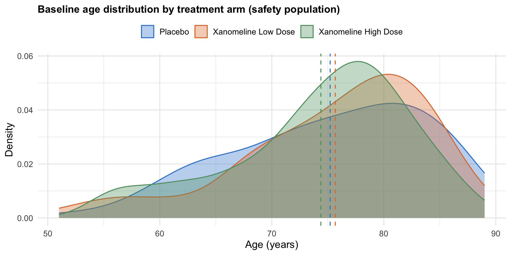
Here is the question the table answers, drawn as a picture — the age distribution by arm, computed from the ADSL we summarize below:
The three curves sit almost on top of one another — the arms are balanced on age, which is exactly the reassurance the demographic table exists to provide. By the end of this lesson you will have produced that summary as a formal table, twice. If “ADSL”, “ADaM”, or “treatment arm” are new, start with Create ADSL in R with admiral, which builds the subject-level dataset this table reads from.
What a demographic table is
A demographic table is a summary table: one analysis population, summarized by treatment arm. Its shape is fixed by long-standing convention — the ICH E3 guideline on Clinical Study Reports defines section 14.1, Demographic Data, and the industry Table 14-1.01 numbering follows from it — so every one you ever build has the same anatomy:
| Part | What it is | In this lesson |
|---|---|---|
| Rows | The baseline characteristics being summarized | Age, age group, sex, race |
| Columns | The treatment arms, plus a Total | Placebo · Xanomeline Low · Xanomeline High · All Patients |
| Continuous stats | Descriptive statistics per arm | n, mean (SD), median, min–max |
| Categorical stats | Counts within each arm | n (%) per category |
| Column header (N=) | The population size of each arm | The “big N” — every percentage’s denominator |
Two conventions decide whether a table is right:
- Continuous variables get distribution statistics, categorical variables get counts. Age is continuous, so it reports a mean and spread; sex and race are categorical, so they report counts and percentages. Mixing these up (a “mean” for sex) is the classic beginner error — both engines below pick the right summary from the variable’s type, which is exactly why you use them instead of hand-rolling
aggregate(). - The percentage denominator is the column N, not the grand total. A 90% for “WHITE” in the Placebo column means 90% of the Placebo arm, not 90% of everyone. Getting this right is what makes the columns add up.
The data
We use the ADSL (Subject-Level Analysis Dataset) shipped in pharmaverseadam — one row per subject from the synthetic CDISC pilot study, already carrying the treatment arm, demographics, and population flags a demographic table needs. We summarize the safety population (SAFFL == "Y"), the standard population for a baseline table: it drops the 52 screen-failure subjects who were never dosed, leaving the three real treatment arms.
library(dplyr, warn.conflicts = FALSE)
library(pharmaverseadam)

adsl <- pharmaverseadam::adsl %>%
  filter(SAFFL == "Y") %>%
  mutate(
    # Order the arms the way the table should read (placebo first), and make the
    # categorical variables factors so their levels display in a controlled order.
    TRT01P = factor(TRT01P,
      levels = c("Placebo", "Xanomeline Low Dose", "Xanomeline High Dose")),
    AGEGR1 = factor(AGEGR1, levels = c("18-64", ">64")),
    SEX    = factor(SEX, levels = c("F", "M")),
    RACE   = factor(RACE)
  )

adsl %>%
  select(USUBJID, TRT01P, AGE, AGEGR1, SEX, RACE) %>%
  head(5)
# A tibble: 5 × 6
USUBJID TRT01P AGE AGEGR1 SEX RACE
<chr> <fct> <dbl> <fct> <fct> <fct>
1 01-701-1015 Placebo 63 18-64 F WHITE
2 01-701-1023 Placebo 64 18-64 M WHITE
3 01-701-1028 Xanomeline High Dose 71 >64 M WHITE
4 01-701-1033 Xanomeline Low Dose 74 >64 M WHITE
5 01-701-1034 Xanomeline High Dose 77 >64 F WHITEOrdering the arms as factors matters: it fixes the column order of the table (placebo first, then ascending dose), instead of letting it fall alphabetical. The four characteristics we will summarize are AGE (continuous), AGEGR1 (age band), SEX, and RACE (all categorical).
Build it fast with gtsummary
gtsummary::tbl_summary() turns a data frame into a publication-ready summary table in a single call. You hand it the variables, tell it to split by the treatment arm, and it picks a sensible summary for each variable type automatically. Three additions make it submission-shaped: add_overall() appends the Total column, label gives each row a human-readable name, and statistic pins the exact summaries the convention asks for.
library(gtsummary)

adsl %>%
  select(TRT01P, AGE, AGEGR1, SEX, RACE) %>%
  tbl_summary(
    by = TRT01P,                                  # one column per treatment arm
    label = list(                                 # readable row labels
      AGE    ~ "Age (years)",
      AGEGR1 ~ "Age group",
      SEX    ~ "Sex",
      RACE   ~ "Race"
    ),
    statistic = list(
      all_continuous()  ~ "{mean} ({sd})",        # continuous: mean (SD)
      all_categorical() ~ "{n} ({p}%)"            # categorical: n (percent)
    ),
    digits = all_continuous() ~ 1
  ) %>%
  add_overall(last = TRUE) %>%                    # the Total column, on the right
  modify_header(label ~ "**Characteristic**") %>%
bold_labels()| Characteristic | Placebo N = 861 |
Xanomeline Low Dose N = 841 |
Xanomeline High Dose N = 841 |
Overall N = 2541 |
|---|---|---|---|---|
| Age (years) | 75.2 (8.6) | 75.7 (8.3) | 74.4 (7.9) | 75.1 (8.2) |
| Age group | ||||
| 18-64 | 14 (16%) | 8 (9.5%) | 11 (13%) | 33 (13%) |
| >64 | 72 (84%) | 76 (90%) | 73 (87%) | 221 (87%) |
| Sex | ||||
| F | 53 (62%) | 50 (60%) | 40 (48%) | 143 (56%) |
| M | 33 (38%) | 34 (40%) | 44 (52%) | 111 (44%) |
| Race | ||||
| AMERICAN INDIAN OR ALASKA NATIVE | 0 (0%) | 0 (0%) | 1 (1.2%) | 1 (0.4%) |
| BLACK OR AFRICAN AMERICAN | 8 (9.3%) | 6 (7.1%) | 9 (11%) | 23 (9.1%) |
| WHITE | 78 (91%) | 78 (93%) | 74 (88%) | 230 (91%) |
| 1 Mean (SD); n (%) | ||||
Read the output the way a reviewer does. The header row carries each arm’s N — N = 86 for Placebo — and every percentage below is out of that N. Age (years) reports 75.2 (8.6): a mean of 75.2 years with a standard deviation of 8.6 in the Placebo arm. Sex and Race report counts and column percentages, so the 53 (62%) females in Placebo means 62% of the 86 Placebo subjects. The Total column on the right pools all 254 subjects. That is a complete, correct demographic table — built in one function call, rendered straight to HTML.
tbl_summary() is the right tool when you want a fast, good-looking table for a report, a Quarto document, or exploration. What it is not built for is the validated, paginated, RTF output a regulatory submission needs — which is where rtables and tern come in.
Build it submission-grade with rtables and tern
In regulated work the table is built from an explicit layout — a pre-data description of the table’s structure — which is then applied to the data. This separation is what makes the output auditable and reusable: the same layout can be re-run on any dataset, paginated, and exported to RTF. rtables provides the layout engine; tern adds the clinical analysis functions on top. The demographic table is tern’s analyze_vars() dropped into an rtables layout.
You read the layout top-to-bottom as a recipe: start a table, split the columns by treatment arm, add the Total column and the column counts, then analyze the chosen variables. Nothing is computed until build_table() applies the layout to the data.
library(rtables)
library(tern)

# 1. Describe the table layout (pre-data — no numbers yet)
lyt <- basic_table(
    title    = "Table 14-1.01",
    subtitles = "Demographic and Baseline Characteristics (Safety Population)"
  ) %>%
  split_cols_by("TRT01P") %>%                       # one column per arm
  add_overall_col("All Patients") %>%               # the Total column
  add_colcounts() %>%                               # the (N=xx) header row
  analyze_vars(
    vars       = c("AGE", "AGEGR1", "SEX", "RACE"),
    var_labels = c("Age (years)", "Age group", "Sex", "Race"),
    .stats     = c("n", "mean_sd", "median", "range", "count_fraction"),
    .formats   = c(mean_sd = "xx.x (xx.x)", median = "xx.x", range = "xx.x - xx.x")
  )

# 2. Apply the layout to the data to produce the table
build_table(lyt, df = adsl)
Table 14-1.01
Demographic and Baseline Characteristics (Safety Population)
————————————————————————————————————————————————————————————————————————————————————————————————————————————
Placebo Xanomeline Low Dose Xanomeline High Dose All Patients
(N=86) (N=84) (N=84) (N=254)
————————————————————————————————————————————————————————————————————————————————————————————————————————————
Age (years)
n 86 84 84 254
Mean (SD) 75.2 (8.6) 75.7 (8.3) 74.4 (7.9) 75.1 (8.2)
Median 76.0 77.5 76.0 77.0
Min - Max 52.0 - 89.0 51.0 - 88.0 56.0 - 88.0 51.0 - 89.0
Age group
n 86 84 84 254
18-64 14 (16.3%) 8 (9.5%) 11 (13.1%) 33 (13%)
>64 72 (83.7%) 76 (90.5%) 73 (86.9%) 221 (87%)
Sex
n 86 84 84 254
F 53 (61.6%) 50 (59.5%) 40 (47.6%) 143 (56.3%)
M 33 (38.4%) 34 (40.5%) 44 (52.4%) 111 (43.7%)
Race
n 86 84 84 254
AMERICAN INDIAN OR ALASKA NATIVE 0 0 1 (1.2%) 1 (0.4%)
BLACK OR AFRICAN AMERICAN 8 (9.3%) 6 (7.1%) 9 (10.7%) 23 (9.1%)
WHITE 78 (90.7%) 78 (92.9%) 74 (88.1%) 230 (90.6%) The output is deliberately plain — fixed-width, monospaced, footnote- and pagination-ready — because that is what a submission table is. Walk down it: under Age (years) you get n, Mean (SD), Median, and Min - Max per arm; under Sex and Race, n and the count (fraction%) for each category. Compare the numbers to the gtsummary table above — Placebo age 75.2 (8.6), 53 (61.6%) female — they are identical, because both engines summarize the same ADSL. What differs is the machinery: tern produced a layout you can validate, reuse on the next dataset, paginate, and hand to rtables’s RTF exporter for the submission package.
The power of the layout shows when you reuse it. Because lyt is a description, not a result, the same demographic table for any subgroup is one more build_table() — no re-specification:
# The same layout, applied to the female subjects only
build_table(lyt, df = adsl %>% filter(SEX == "F"))
Table 14-1.01
Demographic and Baseline Characteristics (Safety Population)
————————————————————————————————————————————————————————————————————————————————————————————————————————————
Placebo Xanomeline Low Dose Xanomeline High Dose All Patients
(N=53) (N=50) (N=40) (N=143)
————————————————————————————————————————————————————————————————————————————————————————————————————————————
Age (years)
n 53 50 40 143
Mean (SD) 76.4 (8.7) 75.7 (8.1) 74.7 (7.7) 75.7 (8.2)
Median 78.0 77.5 76.0 77.0
Min - Max 59.0 - 89.0 54.0 - 87.0 56.0 - 88.0 54.0 - 89.0
Age group
n 53 50 40 143
18-64 9 (17%) 5 (10%) 5 (12.5%) 19 (13.3%)
>64 44 (83%) 45 (90%) 35 (87.5%) 124 (86.7%)
Sex
n 53 50 40 143
F 53 (100%) 50 (100%) 40 (100%) 143 (100%)
M 0 0 0 0
Race
n 53 50 40 143
AMERICAN INDIAN OR ALASKA NATIVE 0 0 0 0
BLACK OR AFRICAN AMERICAN 5 (9.4%) 6 (12%) 6 (15%) 17 (11.9%)
WHITE 48 (90.6%) 44 (88%) 34 (85%) 126 (88.1%) Which engine, when
Both engines are correct; they serve different points in the workflow. Use this as the decision cue:
| gtsummary | rtables + tern | |
|---|---|---|
| Best for | Fast exploration, Quarto/HTML reports, manuscripts | Regulatory submission outputs |
| Mental model | One call does everything | Build a reusable layout, then apply it |
| Output | Polished HTML / gt / flextable | Monospaced, paginated, RTF-ready |
| Reuse on a new dataset | Re-call the function | Re-run the same layout object |
| Industry role | Widely used in academia + early analysis | The pharma standard for validated TLFs |
In practice many teams use both: gtsummary to explore and to draft a table fast, then rtables/tern for the version that goes into the validated submission. They are complementary, not competing.
🟢 With an AI agent
Ask Prova “how do I add a p-value column comparing the treatment arms to my gtsummary demographic table?” — it answers grounded in this pillar’s lessons, with runnable code you can try on the example pharmaverse data. The runtime is the judge. Ask Prova →
Common issues
Every percentage is computed out of the wrong total. If your categorical percentages look too small, you are almost certainly summarizing the whole dataset instead of splitting by arm. In gtsummary the by = TRT01P argument is what makes percentages column-wise; in tern, split_cols_by("TRT01P") does it. Without the split, you get one column and percentages out of the grand total.
Screen failures inflate the counts. pharmaverseadam::adsl keeps the 52 screen-failure subjects (arm "Screen Failure"), who were randomized-out and never dosed. A demographic table summarizes an analysis population, so filter to it first — filter(SAFFL == "Y") for the safety population. Skip the filter and you get a spurious fourth “Screen Failure” column and wrong arm totals.
A categorical variable is summarized as continuous (or vice versa). Both engines choose the summary from the column’s type. A character or factor is treated as categorical (counts); a numeric is treated as continuous (mean/median). If AGEGR1 came through as the string it is stored as, that is fine — but a numeric coded variable (e.g. a 0/1 flag stored as a number) will be mean-summarized unless you make it a factor first. When in doubt, factor() the categorical variables before summarizing, as we did with SEX and AGEGR1.
Frequently asked questions
NoteWhat is a demographic table (Table 1) in a clinical trial?
It is the demographic and baseline-characteristics table that summarizes the trial population by treatment arm — typically age, sex, race, and key baseline measures down the rows, with one column per arm plus a Total. In a Clinical Study Report it is usually numbered Table 14-1.01 (the numbering convention from the ICH E3 guideline); in a journal it is “Table 1”. Its job is to show whether the arms were comparable at baseline.
NoteHow do I make a demographic table in R?
Two common ways. The fast way is gtsummary::tbl_summary(): tbl_summary(by = TRT01P) plus add_overall() gives a labelled HTML table in one call. The submission-grade way is rtables + tern: build a layout with basic_table() |> split_cols_by("TRT01P") |> analyze_vars(...) and apply it with build_table(). Both are worked through above on public pharmaverse data.
NoteWhat is the difference between gtsummary and rtables/tern?
gtsummary is a one-call, general-purpose summary-table package that renders polished HTML — ideal for exploration, manuscripts, and reports. rtables/tern is the pharma layout engine: you describe a reusable layout that is applied to data, producing the monospaced, paginated, RTF-exportable output a regulatory submission requires. Use gtsummary to move fast; use rtables/tern for validated submission TLFs. Many teams use both.
NoteWhich statistics go in a demographic table?
By convention, continuous variables (like age) report n, mean (SD), median, and min–max, and categorical variables (like sex and race) report n (%) — where the percentage denominator is the column’s population size (the “big N” in the header), not the grand total. Both engines in this lesson pick the right summary from each variable’s type automatically.
NoteWhy does my table have a “Screen Failure” column or wrong totals?
Because the ADSL still contains screen-failure subjects. A demographic table summarizes a single analysis population, so filter to it before summarizing — filter(SAFFL == "Y") for the safety population drops the 52 never-dosed screen failures and leaves the three real treatment arms with the correct column counts.
NoteCan I export the rtables demographic table to RTF for a submission?
Yes — that is the reason to use it. rtables outputs are designed to paginate and export to RTF (and TXT) for the submission package via its exporters. Because the table is built from a reusable layout object, the same layout can be re-applied to a new dataset or a subgroup and re-exported, which is what makes it auditable and validation-friendly. (The export and pagination step is covered in the Pro depth of this series.)
Test your understanding
ImportantYour turn: add region to the demographic table
Using the adsl object built in this lesson, add a geographic region characteristic to the gtsummary demographic table. Derive a REGION factor that is "North America" when COUNTRY is "USA" or "CAN" and "Rest of World" otherwise, label it "Region", and include it as a new row split by treatment arm with a Total column.
TipHint
Create the new column with mutate() + if_else() on COUNTRY, wrap it in factor() so it is treated as categorical, then add REGION to the select() and to the label list in tbl_summary(). The percentages will be column-wise automatically because of by = TRT01P.
TipSolution
library(dplyr)
library(gtsummary)

adsl %>%
  mutate(REGION = factor(if_else(COUNTRY %in% c("USA", "CAN"),
                                 "North America", "Rest of World"))) %>%
  select(TRT01P, AGE, SEX, REGION) %>%
  tbl_summary(
    by = TRT01P,
    label = list(AGE ~ "Age (years)", SEX ~ "Sex", REGION ~ "Region"),
    statistic = list(all_continuous() ~ "{mean} ({sd})",
                     all_categorical() ~ "{n} ({p}%)"),
    digits = all_continuous() ~ 1
  ) %>%
  add_overall(last = TRUE) %>%
  modify_header(label ~ "**Characteristic**")
REGION appears as a new categorical block with n (%) per arm. In the CDISC pilot every subject is in the USA, so the table shows a single “North America” row at 100% in each arm — a reminder to always check that a derived grouping actually varies before reading anything into it.
NoteQuick check: in a demographic table, what is each categorical percentage out of?
A. The grand total of all subjects in the trial B. The number of subjects in that column’s treatment arm (the column N) C. The number of subjects with a non-missing value for that variable
TipShow answer
B. Each categorical n (%) is computed within its column — the percentage denominator is the arm’s population size, shown as the N = in the column header. That is why the counts in a column add up to that column’s N, and why splitting by treatment arm (by = TRT01P / split_cols_by("TRT01P")) is what makes the percentages meaningful. (C describes how missing values are handled, a separate setting; A is the error you get if you forget to split by arm.)
Conclusion
The demographic table is the first output of the TLF workflow and the simplest to reason about: one analysis population, summarized by treatment arm, with the right statistic for each variable type. R gives you two engines for it. gtsummary::tbl_summary() builds it in one call and renders polished HTML — perfect for exploration and reports. rtables + tern build it from an explicit, reusable layout (basic_table() |> split_cols_by() |> analyze_vars() |> build_table()) that validates, paginates, and exports to RTF — the engine a submission needs. They produce the same numbers; they serve different ends. Get the population and the column split right, and every count in your Table 14-1.01 is right.
Note
This lesson is reproducible: every result on this page was produced by the code shown — copy any block and run it to reproduce them. The runtime is the judge.
Reuse
Citation
BibTeX citation:
@online{2026,
  author = {},
  title = {The Rtables {Demographic} {Table:} {Build} {Table} 1 in {R}
    {Two} {Ways}},
  date = {2026-06-30},
  url = {https://www.datanovia.com/learn/pharma-clinical/04-tlf-generation/demographic-table-rtables},
  langid = {en}
}
For attribution, please cite this work as:
“The Rtables Demographic Table: Build Table 1 in R Two
Ways.” 2026. June 30. https://www.datanovia.com/learn/pharma-clinical/04-tlf-generation/demographic-table-rtables.