Statistical Modeling with lm() and glm() in R

Introduction

Statistical modeling is a cornerstone of data analysis in R. This tutorial will walk you through how to build regression models using lm() for linear regression and glm() for generalized linear models, such as logistic regression. In addition to model fitting, we will cover techniques for diagnosing model performance, interpreting results, and exploring advanced modeling techniques such as interaction terms and polynomial regression.

1. Linear Modeling with lm()

The lm() function fits a linear model by minimizing the sum of squared errors. We’ll start with a simple example using the mtcars dataset to predict miles-per-gallon (mpg) based on car weight (wt).

data("mtcars")
lm_model <- lm(mpg ~ wt, data = mtcars)
summary(lm_model)

Call:
lm(formula = mpg ~ wt, data = mtcars)

Residuals:
    Min      1Q  Median      3Q     Max 
-4.5432 -2.3647 -0.1252  1.4096  6.8727 

Coefficients:
            Estimate Std. Error t value Pr(>|t|)    
(Intercept)  37.2851     1.8776  19.858  < 2e-16 ***
wt           -5.3445     0.5591  -9.559 1.29e-10 ***
---
Signif. codes:  0 '***' 0.001 '**' 0.01 '*' 0.05 '.' 0.1 ' ' 1

Residual standard error: 3.046 on 30 degrees of freedom
Multiple R-squared:  0.7528,    Adjusted R-squared:  0.7446 
F-statistic: 91.38 on 1 and 30 DF,  p-value: 1.294e-10

Interpretation

• Intercept and Coefficient:
  The output shows the intercept and slope (coefficient for wt). For each additional unit of weight, mpg is expected to change by the coefficient value.
• R-squared:
  Indicates how much of the variability in mpg is explained by the model.
• P-values:
  Assess the statistical significance of the predictors.

2. Generalized Linear Modeling with glm()

The glm() function extends linear models to accommodate non-normal error distributions. A common use is logistic regression for binary outcomes. Here, we predict transmission type (am, where 0 = automatic, 1 = manual) based on car weight (wt).

glm_model <- glm(am ~ wt, data = mtcars, family = binomial)
summary(glm_model)

Call:
glm(formula = am ~ wt, family = binomial, data = mtcars)

Coefficients:
            Estimate Std. Error z value Pr(>|z|)   
(Intercept)   12.040      4.510   2.670  0.00759 **
wt            -4.024      1.436  -2.801  0.00509 **
---
Signif. codes:  0 '***' 0.001 '**' 0.01 '*' 0.05 '.' 0.1 ' ' 1

(Dispersion parameter for binomial family taken to be 1)

    Null deviance: 43.230  on 31  degrees of freedom
Residual deviance: 19.176  on 30  degrees of freedom
AIC: 23.176

Number of Fisher Scoring iterations: 6

Interpretation

• Coefficients:
  Represent log-odds. Use exp(coef(glm_model)) to obtain odds ratios.
• Family and Link Function:
  The binomial family with a logit link is used for binary outcomes.

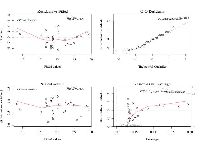
3. Model Diagnostics and Validation

After fitting a model, it’s essential to verify that the model assumptions hold.

Diagnostic Plots for lm()

#| label: lm-diagnostics
par(mfrow = c(2, 2))
plot(lm_model)

Regression model diagnostics

These plots help you assess:

• Residuals vs. Fitted: Checks for non-linearity.
• Normal Q-Q Plot: Evaluates the normality of residuals.
• Scale-Location Plot: Tests for homoscedasticity.
• Residuals vs. Leverage: Identifies influential observations.

Diagnostics for glm()

For generalized linear models, you might use:

• Deviance Residuals: Check model fit.
• Hosmer-Lemeshow Test: Assess goodness-of-fit (requires additional packages).
• ROC Curve: Evaluate classification performance.

4. Interpreting and Visualizing Model Results

Understanding your model’s output is critical for drawing meaningful conclusions.

Interpreting lm() Results

• Coefficients:
  Determine the relationship between predictors and the outcome.
• Confidence Intervals:
  Use confint(lm_model) to assess uncertainty in estimates.

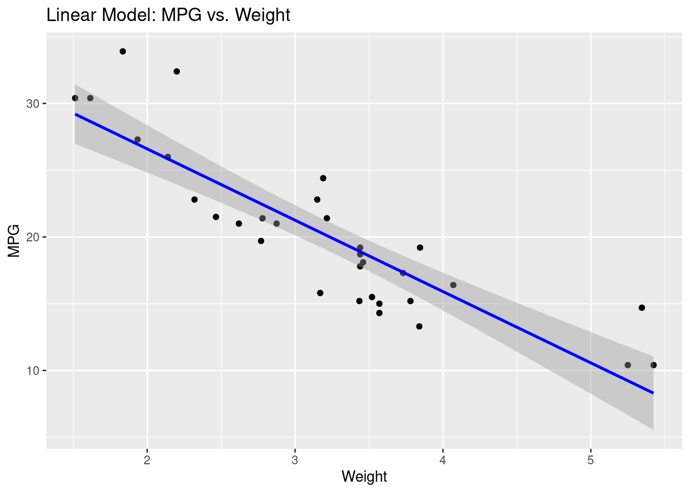
Visualizing Predictions

library(ggplot2)
ggplot(mtcars, aes(x = wt, y = mpg)) +
  geom_point() +
  geom_smooth(method = "lm", se = TRUE, color = "blue") +
  labs(title = "Linear Model: MPG vs. Weight", x = "Weight", y = "MPG")

Interpreting glm() Results

• Odds Ratios:
  Calculate using exp(coef(glm_model)) to understand the effect on the probability scale.
• Predicted Probabilities:
  Use predict(glm_model, type = "response") to get probabilities for the binary outcome.

5. Advanced Modeling Techniques

Enhance your models by incorporating additional predictors or transforming variables.

Interaction Terms

Include interactions to explore whether the effect of one predictor depends on another.

interaction_model <- lm(mpg ~ wt * cyl, data = mtcars)
summary(interaction_model)

Call:
lm(formula = mpg ~ wt * cyl, data = mtcars)

Residuals:
    Min      1Q  Median      3Q     Max 
-4.2288 -1.3495 -0.5042  1.4647  5.2344 

Coefficients:
            Estimate Std. Error t value Pr(>|t|)    
(Intercept)  54.3068     6.1275   8.863 1.29e-09 ***
wt           -8.6556     2.3201  -3.731 0.000861 ***
cyl          -3.8032     1.0050  -3.784 0.000747 ***
wt:cyl        0.8084     0.3273   2.470 0.019882 *  
---
Signif. codes:  0 '***' 0.001 '**' 0.01 '*' 0.05 '.' 0.1 ' ' 1

Residual standard error: 2.368 on 28 degrees of freedom
Multiple R-squared:  0.8606,    Adjusted R-squared:  0.8457 
F-statistic: 57.62 on 3 and 28 DF,  p-value: 4.231e-12

Polynomial Regression

Model non-linear relationships by adding polynomial terms.

poly_model <- lm(mpg ~ poly(wt, 2), data = mtcars)
summary(poly_model)

Call:
lm(formula = mpg ~ poly(wt, 2), data = mtcars)

Residuals:
   Min     1Q Median     3Q    Max 
-3.483 -1.998 -0.773  1.462  6.238 

Coefficients:
             Estimate Std. Error t value Pr(>|t|)    
(Intercept)   20.0906     0.4686  42.877  < 2e-16 ***
poly(wt, 2)1 -29.1157     2.6506 -10.985 7.52e-12 ***
poly(wt, 2)2   8.6358     2.6506   3.258  0.00286 ** 
---
Signif. codes:  0 '***' 0.001 '**' 0.01 '*' 0.05 '.' 0.1 ' ' 1

Residual standard error: 2.651 on 29 degrees of freedom
Multiple R-squared:  0.8191,    Adjusted R-squared:  0.8066 
F-statistic: 65.64 on 2 and 29 DF,  p-value: 1.715e-11

Model Comparison

Use criteria such as AIC (Akaike Information Criterion) to compare different models.

model1 <- lm(mpg ~ wt, data = mtcars)
model2 <- lm(mpg ~ wt + cyl, data = mtcars)
AIC(model1, model2)

       df      AIC
model1  3 166.0294
model2  4 156.0101

Conclusion

This tutorial provided a comprehensive overview of statistical modeling in R using lm() and glm(). You learned how to fit models, diagnose issues, interpret outputs, and enhance your models with advanced techniques. By integrating these methods, you can build robust statistical models that yield insightful and reliable results.

Further Reading

• Data Wrangling with dplyr
• Data Visualization with ggplot2
• Tidyverse for Data Science
• Error Handling in R

Happy coding, and enjoy building robust models with R!

Explore More Articles

Note

Here are more articles from the same category to help you dive deeper into the topic.