This article describes how to do a paired t-test in R (or in Rstudio). Note that the paired t-test is also referred as dependent t-test, related samples t-test, matched pairs t test or paired sample t test.
You will learn how to:
- Perform the paired t-test in R using the following functions :
t_test()[rstatix package]: the result is a data frame for easy plotting using theggpubrpackage.t.test()[stats package]: R base function.
- Interpret and report the paired t-test
- Add p-values and significance levels to a plot
- Calculate and report the paired t-test effect size using Cohen’s d. The
dstatistic redefines the difference in means as the number of standard deviations that separates those means. T-test conventional effect sizes, proposed by Cohen, are: 0.2 (small effect), 0.5 (moderate effect) and 0.8 (large effect) (Cohen 1998).
Contents:
Related Book
Practical Statistics in R II - Comparing Groups: Numerical VariablesPrerequisites
Make sure you have installed the following R packages:
tidyversefor data manipulation and visualizationggpubrfor creating easily publication ready plotsrstatixprovides pipe-friendly R functions for easy statistical analyses.datarium: contains required data sets for this chapter.
Start by loading the following required packages:
library(tidyverse)
library(ggpubr)
library(rstatix)
Demo data
Here, we’ll use a demo dataset mice2 [datarium package], which contains the weight of 10 mice before and after the treatment.
# Wide format
data("mice2", package = "datarium")
head(mice2, 3)
## id before after
## 1 1 187 430
## 2 2 194 404
## 3 3 232 406# Transform into long data:
# gather the before and after values in the same column
mice2.long <- mice2 %>%
gather(key = "group", value = "weight", before, after)
head(mice2.long, 3)## id group weight
## 1 1 before 187
## 2 2 before 194
## 3 3 before 232We want to know, if there is any significant difference in the mean weights after treatment?
Summary statistics
Compute some summary statistics (mean and sd) by groups:
mice2.long %>%
  group_by(group) %>%
  get_summary_stats(weight, type = "mean_sd")
## # A tibble: 2 x 5
## group variable n mean sd
## <chr> <chr> <dbl> <dbl> <dbl>
## 1 after weight 10 400. 30.1
## 2 before weight 10 201. 20.0Calculation
Using the R base function
There are two options for computing the independent t-test depending whether the two groups data are saved either in two different vectors or in a data frame.
Option 1. The data are saved in two different numeric vectors:
# Save the data in two different vector
before <- mice2$before
after <- mice2$after
# Compute t-test
res <- t.test(before, after, paired = TRUE)
res
##
## Paired t-test
##
## data: before and after
## t = -30, df = 9, p-value = 1e-09
## alternative hypothesis: true difference in means is not equal to 0
## 95 percent confidence interval:
## -217 -182
## sample estimates:
## mean of the differences
## -199Option 2. The data are saved in a data frame.
# Compute t-test
res <- t.test(weight ~ group, data = mice2.long, paired = TRUE)
res
As you can see, the two methods give the same results.
In the result above :
tis the t-test statistic value (t = -25.55),dfis the degrees of freedom (df= 9),p-valueis the significance level of the t-test (p-value = 1.03910^{-9}).conf.intis the confidence interval of the mean of the differences at 95% (conf.int = [-217.1442, -181.8158]);sample estimatesis the mean of the differences (mean = -199.48).
Using the rstatix package
We’ll use the pipe-friendly t_test() function [rstatix package], a wrapper around the R base function t.test(). The results can be easily added to a plot using the ggpubr R package.
stat.test <- mice2.long  %>%
  t_test(weight ~ group, paired = TRUE) %>%
  add_significance()
stat.test
## # A tibble: 1 x 9
## .y. group1 group2 n1 n2 statistic df p p.signif
## <chr> <chr> <chr> <int> <int> <dbl> <dbl> <dbl> <chr>
## 1 weight after before 10 10 25.5 9 0.00000000104 ****The results above show the following components:
.y.: the y variable used in the test.group1,group2: the compared groups in the pairwise tests.statistic: Test statistic used to compute the p-value.df: degrees of freedom.p: p-value.
Note that, you can obtain a detailed result by specifying the option detailed = TRUE.
mice2.long %>%
  t_test(weight ~ group, paired = TRUE, detailed = TRUE) %>%
  add_significance()
## # A tibble: 1 x 14
## estimate .y. group1 group2 n1 n2 statistic p df conf.low conf.high method alternative p.signif
## <dbl> <chr> <chr> <chr> <int> <int> <dbl> <dbl> <dbl> <dbl> <dbl> <chr> <chr> <chr>
## 1 199. weight after before 10 10 25.5 0.00000000104 9 182. 217. T-test two.sided ****Interpretation
The p-value of the test is 1.0410^{-9}, which is less than the significance level alpha = 0.05. We can then reject null hypothesis and conclude that the average weight of the mice before treatment is significantly different from the average weight after treatment with a p-value = 1.0410^{-9}.
Effect size
The effect size for a paired-samples t-test can be calculated by dividing the mean difference by the standard deviation of the difference, as shown below.
Cohen’s d formula:
\[
d = \frac{mean_D}{SD_D}
\]
Where D is the differences of the paired samples values.
Calculation:
mice2.long %>% cohens_d(weight ~ group, paired = TRUE)## # A tibble: 1 x 7
## .y. group1 group2 effsize n1 n2 magnitude
## * <chr> <chr> <chr> <dbl> <int> <int> <ord>
## 1 weight after before 8.08 10 10 largeThere is a large effect size, Cohen’s d = 8.07.
Report
We could report the result as follow: The average weight of mice was significantly increased after treatment, t(9) = 25.5, p < 0.0001, d = 8.07.
Visualize the results:
# Create a box plot
bxp <- ggpaired(mice2.long, x = "group", y = "weight",
         order = c("before", "after"),
         ylab = "Weight", xlab = "Groups")

# Add p-value and significance levels
stat.test <- stat.test %>% add_xy_position(x = "group")
bxp +
  stat_pvalue_manual(stat.test, tip.length = 0) +
  labs(subtitle = get_test_label(stat.test, detailed= TRUE))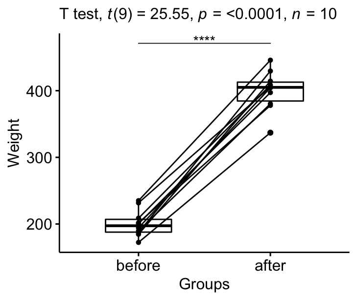
Summary
This article shows how to perform the paired t-test in R/Rstudio using two different ways: the R base function t.test() and the t_test() function in the rstatix package. We also describe how to interpret and report the t-test results.
References
Cohen, J. 1998. Statistical Power Analysis for the Behavioral Sciences. 2nd ed. Hillsdale, NJ: Lawrence Erlbaum Associates.
Recommended for you
This section contains best data science and self-development resources to help you on your path.
Books - Data Science
Our Books
- Practical Guide to Cluster Analysis in R by A. Kassambara (Datanovia)
- Practical Guide To Principal Component Methods in R by A. Kassambara (Datanovia)
- Machine Learning Essentials: Practical Guide in R by A. Kassambara (Datanovia)
- R Graphics Essentials for Great Data Visualization by A. Kassambara (Datanovia)
- GGPlot2 Essentials for Great Data Visualization in R by A. Kassambara (Datanovia)
- Network Analysis and Visualization in R by A. Kassambara (Datanovia)
- Practical Statistics in R for Comparing Groups: Numerical Variables by A. Kassambara (Datanovia)
- Inter-Rater Reliability Essentials: Practical Guide in R by A. Kassambara (Datanovia)
Others
- R for Data Science: Import, Tidy, Transform, Visualize, and Model Data by Hadley Wickham & Garrett Grolemund
- Hands-On Machine Learning with Scikit-Learn, Keras, and TensorFlow: Concepts, Tools, and Techniques to Build Intelligent Systems by Aurelien Géron
- Practical Statistics for Data Scientists: 50 Essential Concepts by Peter Bruce & Andrew Bruce
- Hands-On Programming with R: Write Your Own Functions And Simulations by Garrett Grolemund & Hadley Wickham
- An Introduction to Statistical Learning: with Applications in R by Gareth James et al.
- Deep Learning with R by François Chollet & J.J. Allaire
- Deep Learning with Python by François Chollet
Version:
 Français

This package has made my life easier several times. I was wondering how would you run a paired t-test if you had before and after but for 2 datasets
And is it possible to do it when you have 2 subgroups?