The paired t-test is used to compare the means of two related groups of samples. Put into another words, it’s used in a situation where you have two values (i.e., pair of values) for the same samples.
It is also referred as:
- dependent t-test,
- dependent samples t-test,
- repeated measures t-test,
- related samples t-test,
- paired two sample t-test,
- paired sample t-test and
- t-test for dependent means.
For example, you might want to compare the average weight of 20 mice before and after treatment. The data contain 20 sets of values before treatment and 20 sets of values after treatment from measuring twice the weight of the same mice. In such situations, paired t-test can be used to compare the mean weights before and after treatment.
The procedure of the paired t-test analysis is as follow:
- Calculate the difference (\(d\)) between each pair of value
- Compute the mean (\(m\)) and the standard deviation (\(s\)) of \(d\)
- Compare the average difference to 0. If there is any significant difference between the two pairs of samples, then the mean of d (\(m\)) is expected to be far from 0.
Paired t-test can be used only when the difference \(d\) is normally distributed. This can be checked using the Shapiro-Wilk test.
In this chapter, you will learn the paired t-test formula, as well as, how to:
- Compute the paired t-test in R. The pipe-friendly function
t_test()[rstatix package] will be used. - Check the paired t-test assumptions
- Calculate and report the paired t-test effect size using the Cohen’s d. The
dstatistic redefines the difference in means as the number of standard deviations that separates those means. T-test conventional effect sizes, proposed by Cohen, are: 0.2 (small effect), 0.5 (moderate effect) and 0.8 (large effect) (Cohen 1998).
Contents:
Related Book
Practical Statistics in R II - Comparing Groups: Numerical VariablesPrerequisites
Make sure you have installed the following R packages:
tidyversefor data manipulation and visualizationggpubrfor creating easily publication ready plotsrstatixprovides pipe-friendly R functions for easy statistical analyses.datarium: contains required data sets for this chapter.
Start by loading the following required packages:
library(tidyverse)
library(ggpubr)
library(rstatix)
Research questions
Typical research questions are:
- whether the mean difference (\(m\)) is equal to 0?
- whether the mean difference (\(m\)) is less than 0?
- whether the mean difference (\(m\)) is greather than 0?
statistical hypotheses
In statistics, we can define the corresponding null hypothesis (\(H_0\)) as follow:
- \(H_0: m = 0\)
- \(H_0: m \leq 0\)
- \(H_0: m \geq 0\)
The corresponding alternative hypotheses (\(H_a\)) are as follow:
- \(H_a: m \ne 0\) (different)
- \(H_a: m > 0\) (greater)
- \(H_a: m < 0\) (less)
Note that:
- Hypotheses 1) are called two-tailed tests
- Hypotheses 2) and 3) are called one-tailed tests
Formula
The paired t-test statistics value can be calculated using the following formula:
\[
t = \frac{m}{s/\sqrt{n}}
\]
where,
mis the mean differencesnis the sample size (i.e., size of d).sis the standard deviation of d
We can compute the p-value corresponding to the absolute value of the t-test statistics (|t|) for the degrees of freedom (df): \(df = n - 1\).
If the p-value is inferior or equal to 0.05, we can conclude that the difference between the two paired samples are significantly different.
Demo data
Here, we’ll use a demo dataset mice2 [datarium package], which contains the weight of 10 mice before and after the treatment.
# Wide format
data("mice2", package = "datarium")
head(mice2, 3)
## id before after
## 1 1 187 430
## 2 2 194 404
## 3 3 232 406# Transform into long data:
# gather the before and after values in the same column
mice2.long <- mice2 %>%
gather(key = "group", value = "weight", before, after)
head(mice2.long, 3)## id group weight
## 1 1 before 187
## 2 2 before 194
## 3 3 before 232Summary statistics
Compute some summary statistics (mean and sd) by groups:
mice2.long %>%
  group_by(group) %>%
  get_summary_stats(weight, type = "mean_sd")
## # A tibble: 2 x 5
## group variable n mean sd
## <chr> <chr> <dbl> <dbl> <dbl>
## 1 after weight 10 400. 30.1
## 2 before weight 10 201. 20.0Visualization
bxp <- ggpaired(mice2.long, x = "group", y = "weight",
         order = c("before", "after"),
         ylab = "Weight", xlab = "Groups")
bxp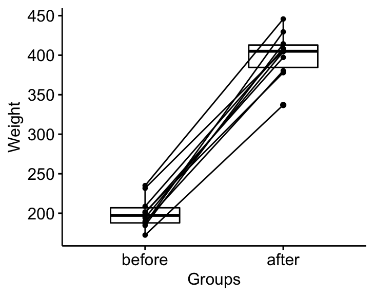
Assumptions and preleminary tests
The paired samples t-test assume the following characteristics about the data:
- the two groups are paired. In our example, this is the case since the data have been collected from measuring twice the weight of the same mice.
- No significant outliers in the difference between the two related groups
- Normality. the difference of pairs follow a normal distribution.
In this section, we’ll perform some preliminary tests to check whether these assumptions are met.
First, start by computing the difference between groups:
mice2 <- mice2 %>% mutate(differences = before - after)
head(mice2, 3)
## id before after differences
## 1 1 187 430 -242
## 2 2 194 404 -210
## 3 3 232 406 -174Identify outliers
Outliers can be easily identified using boxplot methods, implemented in the R function identify_outliers() [rstatix package].
mice2 %>% identify_outliers(differences)## [1] id before after differences is.outlier is.extreme
## <0 rows> (or 0-length row.names)There were no extreme outliers.
Note that, in the situation where you have extreme outliers, this can be due to: 1) data entry errors, measurement errors or unusual values.
You can include the outlier in the analysis anyway if you do not believe the result will be substantially affected. This can be evaluated by comparing the result of the t-test with and without the outlier.
It’s also possible to keep the outliers in the data and perform Wilcoxon test or robust t-test using the WRS2 package.
Check normality assumption
The normality assumption can be checked by computing the Shapiro-Wilk test for each group. If the data is normally distributed, the p-value should be greater than 0.05.
mice2 %>% shapiro_test(differences) ## # A tibble: 1 x 3
## variable statistic p
## <chr> <dbl> <dbl>
## 1 differences 0.968 0.867From the output, the two p-values are greater than the significance level 0.05 indicating that the distribution of the data are not significantly different from the normal distribution. In other words, we can assume the normality.
You can also create QQ plots for each group. QQ plot draws the correlation between a given data and the normal distribution.
ggqqplot(mice2, "differences")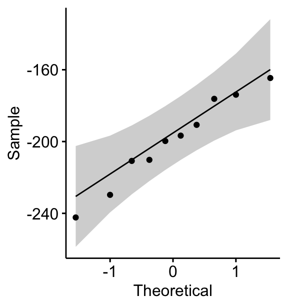
All the points fall approximately along the (45-degree) reference line, for each group. So we can assume normality of the data.
Note that, if your sample size is greater than 50, the normal QQ plot is preferred because at larger sample sizes the Shapiro-Wilk test becomes very sensitive even to a minor deviation from normality.
In the situation where the data are not normally distributed, it’s recommended to use the non parametric Wilcoxon test.
Computation
We want to know, if there is any significant difference in the mean weights after treatment?
We’ll use the pipe-friendly t_test() function [rstatix package], a wrapper around the R base function t.test().
stat.test <- mice2.long  %>%
  t_test(weight ~ group, paired = TRUE) %>%
  add_significance()
stat.test
## # A tibble: 1 x 9
## .y. group1 group2 n1 n2 statistic df p p.signif
## <chr> <chr> <chr> <int> <int> <dbl> <dbl> <dbl> <chr>
## 1 weight after before 10 10 25.5 9 0.00000000104 ****The results above show the following components:
.y.: the y variable used in the test.group1,group2: the compared groups in the pairwise tests.statistic: Test statistic used to compute the p-value.df: degrees of freedom.p: p-value.
Note that, you can obtain a detailed result by specifying the option detailed = TRUE.
To compute one tailed paired t-test, you can specify the option alternative as follow.
- if you want to test whether the average weight before treatment is less than the average weight after treatment, type this:
mice2.long  %>%
t_test(weight ~ group, paired = TRUE, alternative = "less")- Or, if you want to test whether the average weight before treatment is greater than the average weight after treatment, type this
mice2.long  %>%
  t_test(weight ~ group, paired = TRUE, alternative = "greater")
Effect size
The effect size for a paired-samples t-test can be calculated by dividing the mean difference by the standard deviation of the difference, as shown below.
Cohen’s d formula:
\[
d = \frac{mean_D}{SD_D}
\]
Where D is the differences of the paired samples values.
Calculation:
mice2.long %>% cohens_d(weight ~ group, paired = TRUE)## # A tibble: 1 x 7
## .y. group1 group2 effsize n1 n2 magnitude
## * <chr> <chr> <chr> <dbl> <int> <int> <ord>
## 1 weight after before 8.08 10 10 largeThere is a large effect size, Cohen’s d = 8.07.
Report
We could report the result as follow: The average weight of mice was significantly increased after treatment, t(9) = 25.5, p < 0.0001, d = 8.07.
stat.test <- stat.test %>% add_xy_position(x = "group")
bxp +
  stat_pvalue_manual(stat.test, tip.length = 0) +
  labs(subtitle = get_test_label(stat.test, detailed= TRUE))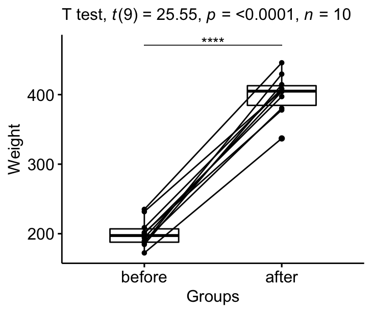
Summary
This article describes the formula and the basics of the paired t-test or dependent t-test. Examples of R codes are provided to check the assumptions, computing the test and the effect size, interpreting and reporting the results.
References
Cohen, J. 1998. Statistical Power Analysis for the Behavioral Sciences. 2nd ed. Hillsdale, NJ: Lawrence Erlbaum Associates.
Recommended for you
This section contains best data science and self-development resources to help you on your path.
Books - Data Science
Our Books
- Practical Guide to Cluster Analysis in R by A. Kassambara (Datanovia)
- Practical Guide To Principal Component Methods in R by A. Kassambara (Datanovia)
- Machine Learning Essentials: Practical Guide in R by A. Kassambara (Datanovia)
- R Graphics Essentials for Great Data Visualization by A. Kassambara (Datanovia)
- GGPlot2 Essentials for Great Data Visualization in R by A. Kassambara (Datanovia)
- Network Analysis and Visualization in R by A. Kassambara (Datanovia)
- Practical Statistics in R for Comparing Groups: Numerical Variables by A. Kassambara (Datanovia)
- Inter-Rater Reliability Essentials: Practical Guide in R by A. Kassambara (Datanovia)
Others
- R for Data Science: Import, Tidy, Transform, Visualize, and Model Data by Hadley Wickham & Garrett Grolemund
- Hands-On Machine Learning with Scikit-Learn, Keras, and TensorFlow: Concepts, Tools, and Techniques to Build Intelligent Systems by Aurelien Géron
- Practical Statistics for Data Scientists: 50 Essential Concepts by Peter Bruce & Andrew Bruce
- Hands-On Programming with R: Write Your Own Functions And Simulations by Garrett Grolemund & Hadley Wickham
- An Introduction to Statistical Learning: with Applications in R by Gareth James et al.
- Deep Learning with R by François Chollet & J.J. Allaire
- Deep Learning with Python by François Chollet
Version:
 Français

No Comments