This article describes how to do a two-sample t-test in R (or in Rstudio). Note the two-sample t-test is also referred as:
- independent t-test,
- independent samples t-test,
- unpaired t-test or
- unrelated t-test.
The independent samples t-test comes in two different forms:
- the standard Student’s t-test, which assumes that the variance of the two groups are equal.
- the Welch’s t-test, which is less restrictive compared to the original Student’s test. This is the test where you do not assume that the variance is the same in the two groups, which results in the fractional degrees of freedom.
The two methods give very similar results unless both the group sizes and the standard deviations are very different.
You will learn how to:
- Perform the independent t-test in R using the following functions :
t_test()[rstatix package]: the result is a data frame for easy plotting using theggpubrpackage.t.test()[stats package]: R base function.
- Interpret and report the two-sample t-test
- Add p-values and significance levels to a plot
- Calculate and report the independent samples t-test effect size using Cohen’s d. The
dstatistic redefines the difference in means as the number of standard deviations that separates those means. T-test conventional effect sizes, proposed by Cohen, are: 0.2 (small effect), 0.5 (moderate effect) and 0.8 (large effect) (Cohen 1998).
Contents:
Related Book
Practical Statistics in R II - Comparing Groups: Numerical VariablesPrerequisites
Make sure you have installed the following R packages:
tidyversefor data manipulation and visualizationggpubrfor creating easily publication ready plotsrstatixprovides pipe-friendly R functions for easy statistical analyses.datarium: contains required data sets for this chapter.
Start by loading the following required packages:
library(tidyverse)
library(ggpubr)
library(rstatix)
Demo data
Demo dataset: genderweight [in datarium package] containing the weight of 40 individuals (20 women and 20 men).
Load the data and show some random rows by groups:
# Load the data
data("genderweight", package = "datarium")
# Show a sample of the data by group
set.seed(123)
genderweight %>% sample_n_by(group, size = 2)
## # A tibble: 4 x 3
## id group weight
## <fct> <fct> <dbl>
## 1 6 F 65.0
## 2 15 F 65.9
## 3 29 M 88.9
## 4 37 M 77.0We want to know, whether the average weights are different between groups.
Summary statistics
Compute some summary statistics by groups: mean and sd (standard deviation)
genderweight %>%
  group_by(group) %>%
  get_summary_stats(weight, type = "mean_sd")
## # A tibble: 2 x 5
## group variable n mean sd
## <fct> <chr> <dbl> <dbl> <dbl>
## 1 F weight 20 63.5 2.03
## 2 M weight 20 85.8 4.35Calculation
Recall that, by default, R computes the Welch t-test, which is the safer one. This is the test where you do not assume that the variance is the same in the two groups, which results in the fractional degrees of freedom. If you want to assume the equality of variances (Student t-test), specify the option var.equal = TRUE.
Using the R base function
There are two options for computing the independent t-test depending whether the two groups data are saved either in two different vectors or in a data frame.
Option 1. The data are saved in two different numeric vectors:
# Save the data in two different vector
women_weight <- genderweight %>%
  filter(group == "F") %>%
  pull(weight)
men_weight <- genderweight %>%
  filter(group == "M") %>%
  pull(weight)
# Compute t-test
res <- t.test(women_weight, men_weight)
res
##
## Welch Two Sample t-test
##
## data: women_weight and men_weight
## t = -20, df = 30, p-value <2e-16
## alternative hypothesis: true difference in means is not equal to 0
## 95 percent confidence interval:
## -24.5 -20.1
## sample estimates:
## mean of x mean of y
## 63.5 85.8Option 2. The data are saved in a data frame.
# Compute t-test
res <- t.test(weight ~ group, data = genderweight)
res
##
## Welch Two Sample t-test
##
## data: weight by group
## t = -20, df = 30, p-value <2e-16
## alternative hypothesis: true difference in means is not equal to 0
## 95 percent confidence interval:
## -24.5 -20.1
## sample estimates:
## mean in group F mean in group M
## 63.5 85.8As you can see, the two methods give the same results.
In the result above :
tis the t-test statistic value (t = -20.79),dfis the degrees of freedom (df= 26.872),p-valueis the significance level of the t-test (p-value = 4.29810^{-18}).conf.intis the confidence interval of the means difference at 95% (conf.int = [-24.5314, -20.1235]);sample estimatesis the mean value of the sample (mean = 63.499, 85.826).
Using the rstatix package
We’ll use the pipe-friendly t_test() function [rstatix package], a wrapper around the R base function t.test(). The results can be easily added to a plot using the ggpubr R package.
stat.test <- genderweight %>%
  t_test(weight ~ group) %>%
  add_significance()
stat.test
## # A tibble: 1 x 9
## .y. group1 group2 n1 n2 statistic df p p.signif
## <chr> <chr> <chr> <int> <int> <dbl> <dbl> <dbl> <chr>
## 1 weight F M 20 20 -20.8 26.9 4.30e-18 ****If you want to assume the equality of variances (Student t-test), specify the option var.equal = TRUE:
stat.test2 <- genderweight %>%
  t_test(weight ~ group, var.equal = TRUE) %>%
  add_significance()
stat.test2
The results above show the following components:
.y.: the y variable used in the test.group1,group2: the compared groups in the pairwise tests.statistic: Test statistic used to compute the p-value.df: degrees of freedom.p: p-value.
Note that, you can obtain a detailed result by specifying the option detailed = TRUE.
genderweight %>%
  t_test(weight ~ group, detailed = TRUE) %>%
  add_significance()
## # A tibble: 1 x 16
## estimate estimate1 estimate2 .y. group1 group2 n1 n2 statistic p df conf.low conf.high method alternative p.signif
## <dbl> <dbl> <dbl> <chr> <chr> <chr> <int> <int> <dbl> <dbl> <dbl> <dbl> <dbl> <chr> <chr> <chr>
## 1 -22.3 63.5 85.8 weight F M 20 20 -20.8 4.30e-18 26.9 -24.5 -20.1 T-test two.sided ****Interpretation
The p-value of the test is 4.310^{-18}, which is less than the significance level alpha = 0.05. We can conclude that men’s average weight is significantly different from women’s average weight with a p-value = 4.310^{-18}.
Effect size
Cohen’s d for Student t-test
There are multiple version of Cohen’s d for Student t-test. The most commonly used version of the Student t-test effect size, comparing two groups (\(A\) and \(B\)), is calculated by dividing the mean difference between the groups by the pooled standard deviation.
Cohen’s d formula:
\[
d = \frac{m_A - m_B}{SD_{pooled}}
\]
where,
- \(m_A\) and \(m_B\) represent the mean value of the group A and B, respectively.
- \(n_A\) and \(n_B\) represent the sizes of the group A and B, respectively.
- \(SD_{pooled}\) is an estimator of the pooled standard deviation of the two groups. It can be calculated as follow :
\[
SD_{pooled} = \sqrt{\frac{\sum{(x-m_A)^2}+\sum{(x-m_B)^2}}{n_A+n_B-2}}
\]
Calculation. If the option var.equal = TRUE, then the pooled SD is used when compting the Cohen’s d.
genderweight %>% cohens_d(weight ~ group, var.equal = TRUE)## # A tibble: 1 x 7
## .y. group1 group2 effsize n1 n2 magnitude
## * <chr> <chr> <chr> <dbl> <int> <int> <ord>
## 1 weight F M -6.57 20 20 largeThere is a large effect size, d = 6.57.
Note that, for small sample size (< 50), the Cohen’s d tends to over-inflate results. There exists a Hedge’s Corrected version of the Cohen’s d (Hedges and Olkin 1985), which reduces effect sizes for small samples by a few percentage points. The correction is introduced by multiplying the usual value of d by (N-3)/(N-2.25) (for unpaired t-test) and by (n1-2)/(n1-1.25) for paired t-test; where N is the total size of the two groups being compared (N = n1 + n2).
Cohen’s d for Welch t-test
The Welch test is a variant of t-test used when the equality of variance can’t be assumed. The effect size can be computed by dividing the mean difference between the groups by the “averaged” standard deviation.
Cohen’s d formula:
\[
d = \frac{m_A - m_B}{\sqrt{(Var_1 + Var_2)/2}}
\]
where,
- \(m_A\) and \(m_B\) represent the mean value of the group A and B, respectively.
- \(Var_1\) and \(Var_2\) are the variance of the two groups.
Calculation:
genderweight %>% cohens_d(weight ~ group, var.equal = FALSE)## # A tibble: 1 x 7
## .y. group1 group2 effsize n1 n2 magnitude
## * <chr> <chr> <chr> <dbl> <int> <int> <ord>
## 1 weight F M -6.57 20 20 largeNote that, when group sizes are equal and group variances are homogeneous, Cohen’s d for the standard Student and Welch t-tests are identical.
Report
We could report the result as follow:
The mean weight in female group was 63.5 (SD = 2.03), whereas the mean in male group was 85.8 (SD = 4.3). A Welch two-samples t-test showed that the difference was statistically significant, t(26.9) = -20.8, p < 0.0001, d = 6.57; where, t(26.9) is shorthand notation for a Welch t-statistic that has 26.9 degrees of freedom.
Visualize the results:
# Create a box-plot
bxp <- ggboxplot(
  genderweight, x = "group", y = "weight",
  ylab = "Weight", xlab = "Groups", add = "jitter"
  )

# Add p-value and significance levels
stat.test <- stat.test %>% add_xy_position(x = "group")
bxp +
  stat_pvalue_manual(stat.test, tip.length = 0) +
  labs(subtitle = get_test_label(stat.test, detailed = TRUE))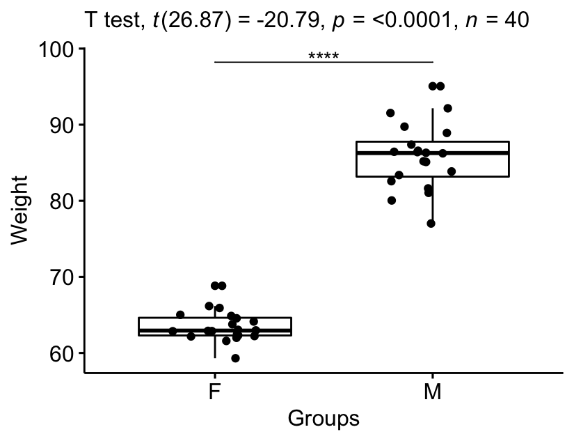
Summary
This article shows how to perform the two-sample t-test in R/Rstudio using two different ways: the R base function t.test() and the t_test() function in the rstatix package. We also describe how to interpret and report the t-test results.
References
Cohen, J. 1998. Statistical Power Analysis for the Behavioral Sciences. 2nd ed. Hillsdale, NJ: Lawrence Erlbaum Associates.
Hedges, Larry, and Ingram Olkin. 1985. “Statistical Methods in Meta-Analysis.” In Stat Med. Vol. 20. doi:10.2307/1164953.
Recommended for you
This section contains best data science and self-development resources to help you on your path.
Books - Data Science
Our Books
- Practical Guide to Cluster Analysis in R by A. Kassambara (Datanovia)
- Practical Guide To Principal Component Methods in R by A. Kassambara (Datanovia)
- Machine Learning Essentials: Practical Guide in R by A. Kassambara (Datanovia)
- R Graphics Essentials for Great Data Visualization by A. Kassambara (Datanovia)
- GGPlot2 Essentials for Great Data Visualization in R by A. Kassambara (Datanovia)
- Network Analysis and Visualization in R by A. Kassambara (Datanovia)
- Practical Statistics in R for Comparing Groups: Numerical Variables by A. Kassambara (Datanovia)
- Inter-Rater Reliability Essentials: Practical Guide in R by A. Kassambara (Datanovia)
Others
- R for Data Science: Import, Tidy, Transform, Visualize, and Model Data by Hadley Wickham & Garrett Grolemund
- Hands-On Machine Learning with Scikit-Learn, Keras, and TensorFlow: Concepts, Tools, and Techniques to Build Intelligent Systems by Aurelien Géron
- Practical Statistics for Data Scientists: 50 Essential Concepts by Peter Bruce & Andrew Bruce
- Hands-On Programming with R: Write Your Own Functions And Simulations by Garrett Grolemund & Hadley Wickham
- An Introduction to Statistical Learning: with Applications in R by Gareth James et al.
- Deep Learning with R by François Chollet & J.J. Allaire
- Deep Learning with Python by François Chollet
Version:
 Français

No Comments