The one-sample t-test, also known as the single-parameter t test or single-sample t-test, is used to compare the mean of one sample to a known standard (or theoretical / hypothetical) mean. Another synonym is the one-way t-test.
Generally, the theoretical mean comes from:
- a previous experiment. For example, comparing whether the mean weight of mice differs from 200 mg, a value determined in a previous study.
- or from an experiment where you have control and treatment conditions. If you express your data as “percent of control”, you can test whether the average value of treatment condition differs significantly from 100.
Note that, the one-sample t-test can be used only, when the data are normally distributed. This can be checked using the Shapiro-Wilk test.
In this article, you will learn the one-sample t-test formula, as well as, how to :
- Calculate the one-sample t-test in R. The pipe-friendly function
t_test()[rstatix package] will be used. - Check the one-sample t-test assumptions
- Calculate and report the one-sample t-test effect size using Cohen’s d. The
dstatistic redefines the difference in means as the number of standard deviations that separates those means. T-test conventional effect sizes, proposed by Cohen, are: 0.2 (small effect), 0.5 (moderate effect) and 0.8 (large effect) (Cohen 1998).
Contents:
Related Book
Practical Statistics in R II - Comparing Groups: Numerical VariablesPrerequisites
Make sure you have installed the following R packages:
tidyversefor data manipulation and visualizationggpubrfor creating easily publication ready plotsrstatixprovides pipe-friendly R functions for easy statistical analyses.datarium: contains required data sets for this chapter.
Start by loading the following required packages:
library(tidyverse)
library(ggpubr)
library(rstatix)
Research questions
Typical research questions are:
- whether the mean (\(m\)) of the sample is equal to the theoretical mean (\(\mu\))?
- whether the mean (\(m\)) of the sample is less than the theoretical mean (\(\mu\))?
- whether the mean (\(m\)) of the sample is greater than the theoretical mean (\(\mu\))?
Statistical hypotheses
In statistics, we can define the corresponding null hypothesis (\(H_0\)) as follow:
- \(H_0: m = \mu\)
- \(H_0: m \leq \mu\)
- \(H_0: m \geq \mu\)
The corresponding alternative hypotheses (\(H_a\)) are as follow:
- \(H_a: m \ne \mu\) (different)
- \(H_a: m > \mu\) (greater)
- \(H_a: m < \mu\) (less)
Note that:
- Hypotheses 1) are called two-tailed tests
- Hypotheses 2) and 3) are called one-tailed tests
Formula
The the one-sample t-test formula can be written as follow:
\[
t = \frac{m-\mu}{s/\sqrt{n}}
\]
where,
- \(m\) is the sample mean
- \(n\) is the sample size
- \(s\) is the sample standard deviation with \(n-1\) degrees of freedom
- \(\mu\) is the theoretical mean
The p-value, corresponding to the absolute value of the t-test statistics (|t|), is computed for the degrees of freedom (df): df = n - 1.
How to interpret the one-sample t-test results?
If the p-value is inferior or equal to the significance level 0.05, we can reject the null hypothesis and accept the alternative hypothesis. In other words, we conclude that the sample mean is significantly different from the theoretical mean.
Demo data
Demo dataset: mice [in datarium package]. Contains the weight of 10 mice:
# Load and inspect the data
data(mice, package = "datarium")
head(mice, 3)
## # A tibble: 3 x 2
## name weight
## <chr> <dbl>
## 1 M_1 18.9
## 2 M_2 19.5
## 3 M_3 23.1Summary statistics
Compute some summary statistics: count (number of subjects), mean and sd (standard deviation)
mice %>% get_summary_stats(weight, type = "mean_sd")## # A tibble: 1 x 4
## variable n mean sd
## <chr> <dbl> <dbl> <dbl>
## 1 weight 10 20.1 1.90Visualization
Create a boxplot to visualize the distribution of mice weights. Add also jittered points to show individual observations. The big dot represents the mean point.
bxp <- ggboxplot(
  mice$weight, width = 0.5, add = c("mean", "jitter"),
  ylab = "Weight (g)", xlab = FALSE
  )
bxp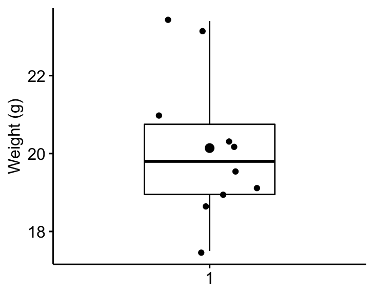
Assumptions and preleminary tests
The one-sample t-test assumes the following characteristics about the data:
- No significant outliers in the data
- Normality. the data should be approximately normally distributed
In this section, we’ll perform some preliminary tests to check whether these assumptions are met.
Identify outliers
Outliers can be easily identified using boxplot methods, implemented in the R function identify_outliers() [rstatix package].
mice %>% identify_outliers(weight)## [1] name weight is.outlier is.extreme
## <0 rows> (or 0-length row.names)There were no extreme outliers.
Note that, in the situation where you have extreme outliers, this can be due to: 1) data entry errors, measurement errors or unusual values.
In this case, you could consider running the non parametric Wilcoxon test.
Check normality assumption
The normality assumption can be checked by computing the Shapiro-Wilk test. If the data is normally distributed, the p-value should be greater than 0.05.
mice %>% shapiro_test(weight)## # A tibble: 1 x 3
## variable statistic p
## <chr> <dbl> <dbl>
## 1 weight 0.923 0.382From the output, the p-value is greater than the significance level 0.05 indicating that the distribution of the data are not significantly different from the normal distribution. In other words, we can assume the normality.
You can also create a QQ plot of the weight data. QQ plot draws the correlation between a given data and the normal distribution.
ggqqplot(mice, x = "weight")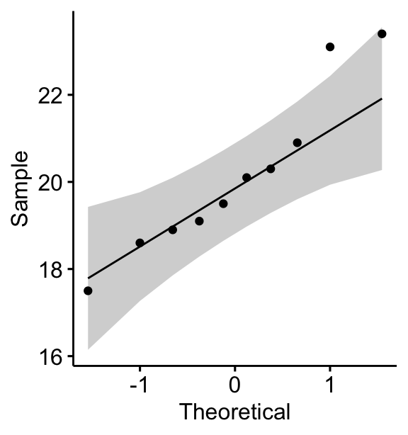
All the points fall approximately along the (45-degree) reference line, for each group. So we can assume normality of the data.
Note that, if your sample size is greater than 50, the normal QQ plot is preferred because at larger sample sizes the Shapiro-Wilk test becomes very sensitive even to a minor deviation from normality.
If the data are not normally distributed, it’s recommended to use a non-parametric test such as the one-sample Wilcoxon signed-rank test. This test is similar to the one-sample t-test, but focuses on the median rather than the mean.
Calculate one-sample t-test in R
We want to know, whether the average weight of the mice differs from 25g (two-tailed test)?
We’ll use the pipe-friendly t_test() function [rstatix package], a wrapper around the R base function t.test().
stat.test <- mice %>% t_test(weight ~ 1, mu = 25)
stat.test
## # A tibble: 1 x 7
## .y. group1 group2 n statistic df p
## * <chr> <chr> <chr> <int> <dbl> <dbl> <dbl>
## 1 weight 1 null model 10 -8.10 9 0.00002The results above show the following components:
.y.: the outcome variable used in the test.group1,group2: generally, the compared groups in the pairwise tests. Here, we have null model (one-sample test).statistic: test statistic (t-value) used to compute the p-value.df: degrees of freedom.p: p-value.
You can obtain a detailed result by specifying the option detailed = TRUE in the function t_test().
Note that:
- if you want to test whether the mean weight of mice is less than 25g (one-tailed test), type this:
mice %>% t_test(weight ~ 1, mu = 25, alternative = "less")- Or, if you want to test whether the mean weight of mice is greater than 25g (one-tailed test), type this:
mice %>% t_test(weight ~ 1, mu = 25, alternative = "greater")To calculate t-test using the R base function, type this:
t.test(mice$weight, mu = 25)Effect size
To calculate an effect size, called Cohen's d, for the one-sample t-test you need to divide the mean difference by the standard deviation of the difference, as shown below. Note that, here: sd(x-mu) = sd(x).
Cohen’s d formula:
\[
d = \frac{m-\mu}{s}
\]
- \(m\) is the sample mean
- \(s\) is the sample standard deviation with \(n-1\) degrees of freedom
- \(\mu\) is the theoretical mean against which the mean of our sample is compared (default value is mu = 0).
Calculation:
mice %>% cohens_d(weight ~ 1, mu = 25)## # A tibble: 1 x 6
## .y. group1 group2 effsize n magnitude
## * <chr> <chr> <chr> <dbl> <int> <ord>
## 1 weight 1 null model 10.6 10 largeRecall that, t-test conventional effect sizes, proposed by Cohen J. (1998), are: 0.2 (small effect), 0.5 (moderate effect) and 0.8 (large effect) (Cohen 1998). As the effect size, d, is 2.56 you can conclude that there is a large effect.
Report
We could report the result as follow:
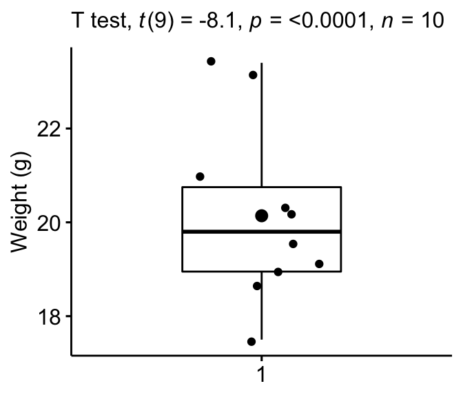
A one-sample t-test was computed to determine whether the recruited mice average weight was different to the population normal mean weight (25g).
The mice weight value were normally distributed, as assessed by Shapiro-Wilk’s test (p > 0.05) and there were no extreme outliers in the data, as assessed by boxplot method.
The measured mice mean weight (20.14 +/- 1.94) was statistically significantly lower than the population normal mean weight 25 (t(9) = -8.1, p < 0.0001, d = 2.56); where t(9) is shorthand notation for a t-statistic that has 9 degrees of freedom.
Create a box plot with p-value:
bxp + labs(
  subtitle = get_test_label(stat.test, detailed = TRUE)
  )
Create a density plot with p-value:
- Red line corresponds to the observed mean
- Blue line corresponds to the theoretical mean
ggdensity(mice, x = "weight", rug = TRUE, fill = "lightgray") +
  scale_x_continuous(limits = c(15, 27)) +
  stat_central_tendency(type = "mean", color = "red", linetype = "dashed") +
  geom_vline(xintercept = 25, color = "blue", linetype = "dashed") +
  labs(subtitle = get_test_label(stat.test,  detailed = TRUE))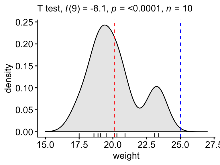
Summary
This article describes the basics and the formula of the on-sample t-test. Additionally, it provides an example for:
- checking the on-sample t-test assumptions,
- calculating the one-sample t-test in R using the
t_test()function [rstatix package], - computing Cohen’s d for one-sample t-test
- Interpreting and reporting the results
References
Cohen, J. 1998. Statistical Power Analysis for the Behavioral Sciences. 2nd ed. Hillsdale, NJ: Lawrence Erlbaum Associates.
Recommended for you
This section contains best data science and self-development resources to help you on your path.
Books - Data Science
Our Books
- Practical Guide to Cluster Analysis in R by A. Kassambara (Datanovia)
- Practical Guide To Principal Component Methods in R by A. Kassambara (Datanovia)
- Machine Learning Essentials: Practical Guide in R by A. Kassambara (Datanovia)
- R Graphics Essentials for Great Data Visualization by A. Kassambara (Datanovia)
- GGPlot2 Essentials for Great Data Visualization in R by A. Kassambara (Datanovia)
- Network Analysis and Visualization in R by A. Kassambara (Datanovia)
- Practical Statistics in R for Comparing Groups: Numerical Variables by A. Kassambara (Datanovia)
- Inter-Rater Reliability Essentials: Practical Guide in R by A. Kassambara (Datanovia)
Others
- R for Data Science: Import, Tidy, Transform, Visualize, and Model Data by Hadley Wickham & Garrett Grolemund
- Hands-On Machine Learning with Scikit-Learn, Keras, and TensorFlow: Concepts, Tools, and Techniques to Build Intelligent Systems by Aurelien Géron
- Practical Statistics for Data Scientists: 50 Essential Concepts by Peter Bruce & Andrew Bruce
- Hands-On Programming with R: Write Your Own Functions And Simulations by Garrett Grolemund & Hadley Wickham
- An Introduction to Statistical Learning: with Applications in R by Gareth James et al.
- Deep Learning with R by François Chollet & J.J. Allaire
- Deep Learning with Python by François Chollet
Version:
 Français

No Comments