This article describes the paired t-test assumptions and provides examples of R code to check whether the assumptions are met before calculating the t-test. This also referred as:
- paired sample t test assumptions,
- assumptions for matched pairs t test and
- assumptions of dependent t test
The procedure of the paired t-test analysis is as follow:
- Calculate the difference (\(d\)) between each pair of value
- Compute the mean (\(m\)) and the standard deviation (\(s\)) of \(d\)
- Compare the average difference to 0. If there is any significant difference between the two pairs of samples, then the mean of d (\(m\)) is expected to be far from 0.
Contents:
Related Book
Practical Statistics in R II - Comparing Groups: Numerical VariablesAssumptions
The paired samples t-test assume the following characteristics about the data:
- the two groups are paired.
- No significant outliers in the difference between the two related groups
- Normality. the difference of pairs follow a normal distribution.
In this section, we’ll perform some preliminary tests to check whether these assumptions are met.
Check paired t-test assumptions in R
Prerequisites
Make sure you have installed the following R packages:
tidyversefor data manipulation and visualizationggpubrfor creating easily publication ready plotsrstatixprovides pipe-friendly R functions for easy statistical analyses.datarium: contains required data sets for this chapter.
Start by loading the following required packages:
library(tidyverse)
library(ggpubr)
library(rstatix)
Demo data
Here, we’ll use a demo dataset mice2 [datarium package], which contains the weight of 10 mice before and after the treatment.
# Wide format
data("mice2", package = "datarium")
head(mice2, 3)
## id before after
## 1 1 187 430
## 2 2 194 404
## 3 3 232 406# Transform into long data:
# gather the before and after values in the same column
mice2.long <- mice2 %>%
gather(key = "group", value = "weight", before, after)
head(mice2.long, 3)## id group weight
## 1 1 before 187
## 2 2 before 194
## 3 3 before 232First, start by computing the difference between groups:
mice2 <- mice2 %>% mutate(differences = before - after)
head(mice2, 3)
## id before after differences
## 1 1 187 430 -242
## 2 2 194 404 -210
## 3 3 232 406 -174Identify outliers
Outliers can be easily identified using boxplot methods, implemented in the R function identify_outliers() [rstatix package].
mice2 %>% identify_outliers(differences)## [1] id before after differences is.outlier is.extreme
## <0 rows> (or 0-length row.names)There were no extreme outliers.
Note that, in the situation where you have extreme outliers, this can be due to: 1) data entry errors, measurement errors or unusual values.
You can include the outlier in the analysis anyway if you do not believe the result will be substantially affected. This can be evaluated by comparing the result of the t-test with and without the outlier.
It’s also possible to keep the outliers in the data and perform Wilcoxon test or robust t-test using the WRS2 package.
Check normality by groups
The normality assumption can be checked by computing the Shapiro-Wilk test for each group. If the data is normally distributed, the p-value should be greater than 0.05.
mice2 %>% shapiro_test(differences) ## # A tibble: 1 x 3
## variable statistic p
## <chr> <dbl> <dbl>
## 1 differences 0.968 0.867From the output, the two p-values are greater than the significance level 0.05 indicating that the distribution of the data are not significantly different from the normal distribution. In other words, we can assume the normality.
You can also create QQ plots for each group. QQ plot draws the correlation between a given data and the normal distribution.
ggqqplot(mice2, "differences")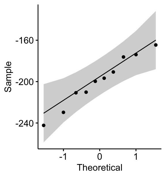
All the points fall approximately along the (45-degree) reference line, for each group. So we can assume normality of the data.
Note that, if your sample size is greater than 50, the normal QQ plot is preferred because at larger sample sizes the Shapiro-Wilk test becomes very sensitive even to a minor deviation from normality.
In the situation where the data are not normally distributed, it’s recommended to use the non parametric Wilcoxon test.
Recommended for you
This section contains best data science and self-development resources to help you on your path.
Books - Data Science
Our Books
- Practical Guide to Cluster Analysis in R by A. Kassambara (Datanovia)
- Practical Guide To Principal Component Methods in R by A. Kassambara (Datanovia)
- Machine Learning Essentials: Practical Guide in R by A. Kassambara (Datanovia)
- R Graphics Essentials for Great Data Visualization by A. Kassambara (Datanovia)
- GGPlot2 Essentials for Great Data Visualization in R by A. Kassambara (Datanovia)
- Network Analysis and Visualization in R by A. Kassambara (Datanovia)
- Practical Statistics in R for Comparing Groups: Numerical Variables by A. Kassambara (Datanovia)
- Inter-Rater Reliability Essentials: Practical Guide in R by A. Kassambara (Datanovia)
Others
- R for Data Science: Import, Tidy, Transform, Visualize, and Model Data by Hadley Wickham & Garrett Grolemund
- Hands-On Machine Learning with Scikit-Learn, Keras, and TensorFlow: Concepts, Tools, and Techniques to Build Intelligent Systems by Aurelien Géron
- Practical Statistics for Data Scientists: 50 Essential Concepts by Peter Bruce & Andrew Bruce
- Hands-On Programming with R: Write Your Own Functions And Simulations by Garrett Grolemund & Hadley Wickham
- An Introduction to Statistical Learning: with Applications in R by Gareth James et al.
- Deep Learning with R by François Chollet & J.J. Allaire
- Deep Learning with Python by François Chollet
Version:
 Français

No Comments