This article describes how to do a one-sample t-test in R (or in Rstudio). You will learn how to:
- Perform a one-sample t-test in R using the following functions :
t_test()[rstatix package]: the result is a data frame for easy plotting using theggpubrpackage.t.test()[stats package]: R base function.
- Interpret and report the one-sample t-test
- Add p-values and significance levels to a plot
- Calculate and report the one-sample t-test effect size using Cohen’s d. The
dstatistic redefines the difference in means as the number of standard deviations that separates those means. T-test conventional effect sizes, proposed by Cohen, are: 0.2 (small effect), 0.5 (moderate effect) and 0.8 (large effect) (Cohen 1998).
Contents:
Related Book
Practical Statistics in R II - Comparing Groups: Numerical VariablesPrerequisites
Make sure you have installed the following R packages:
tidyversefor data manipulation and visualizationggpubrfor creating easily publication ready plotsrstatixprovides pipe-friendly R functions for easy statistical analyses.datarium: contains required data sets for this chapter.
Start by loading the following required packages:
library(tidyverse)
library(ggpubr)
library(rstatix)
Demo data
Demo dataset: mice [in datarium package]. Contains the weight of 10 mice:
# Load and inspect the data
data(mice, package = "datarium")
head(mice, 3)
## # A tibble: 3 x 2
## name weight
## <chr> <dbl>
## 1 M_1 18.9
## 2 M_2 19.5
## 3 M_3 23.1We want to know, whether the average weight of the mice differs from 25g (two-tailed test)?
Summary statistics
Compute some summary statistics: count (number of subjects), mean and sd (standard deviation)
mice %>% get_summary_stats(weight, type = "mean_sd")## # A tibble: 1 x 4
## variable n mean sd
## <chr> <dbl> <dbl> <dbl>
## 1 weight 10 20.1 1.90Calculation
Using the R base function
# One-sample t-test
res <- t.test(mice$weight, mu = 25)

# Printing the results
res
##
## One Sample t-test
##
## data: mice$weight
## t = -8, df = 9, p-value = 2e-05
## alternative hypothesis: true mean is not equal to 25
## 95 percent confidence interval:
## 18.8 21.5
## sample estimates:
## mean of x
## 20.1In the result above :
tis the t-test statistic value (t = -8.105),dfis the degrees of freedom (df= 9),p-valueis the significance level of the t-test (p-value = 1.99510^{-5}).conf.intis the confidence interval of the mean at 95% (conf.int = [18.7835, 21.4965]);sample estimatesis the mean value of the sample (mean = 20.14).
Using the rstatix package
We’ll use the pipe-friendly t_test() function [rstatix package], a wrapper around the R base function t.test(). The results can be easily added to a plot using the ggpubr R package.
stat.test <- mice %>% t_test(weight ~ 1, mu = 25)
stat.test
## # A tibble: 1 x 7
## .y. group1 group2 n statistic df p
## * <chr> <chr> <chr> <int> <dbl> <dbl> <dbl>
## 1 weight 1 null model 10 -8.10 9 0.00002The results above show the following components:
.y.: the outcome variable used in the test.group1,group2: generally, the compared groups in the pairwise tests. Here, we have null model (one-sample test).statistic: test statistic (t-value) used to compute the p-value.df: degrees of freedom.p: p-value.
You can obtain a detailed result by specifying the option detailed = TRUE in the function t_test().
mice %>% t_test(weight ~ 1, mu = 25, detailed = TRUE)## # A tibble: 1 x 12
## estimate .y. group1 group2 n statistic p df conf.low conf.high method alternative
## * <dbl> <chr> <chr> <chr> <int> <dbl> <dbl> <dbl> <dbl> <dbl> <chr> <chr>
## 1 20.1 weight 1 null model 10 -8.10 0.00002 9 18.8 21.5 T-test two.sidedInterpretation
The p-value of the test is 210^{-5}, which is less than the significance level alpha = 0.05. We can conclude that the mean weight of the mice is significantly different from 25g with a p-value = 210^{-5}.
Effect size
To calculate an effect size, called Cohen's d, for the one-sample t-test you need to divide the mean difference by the standard deviation of the difference, as shown below. Note that, here: sd(x-mu) = sd(x).
Cohen’s d formula:
\[
d = \frac{m-\mu}{s}
\]
- \(m\) is the sample mean
- \(s\) is the sample standard deviation with \(n-1\) degrees of freedom
- \(\mu\) is the theoretical mean against which the mean of our sample is compared (default value is mu = 0).
Calculation:
mice %>% cohens_d(weight ~ 1, mu = 25)## # A tibble: 1 x 6
## .y. group1 group2 effsize n magnitude
## * <chr> <chr> <chr> <dbl> <int> <ord>
## 1 weight 1 null model 10.6 10 largeRecall that, t-test conventional effect sizes, proposed by Cohen J. (1998), are: 0.2 (small effect), 0.5 (moderate effect) and 0.8 (large effect) (Cohen 1998). As the effect size, d, is 2.56 you can conclude that there is a large effect.
Reporting
We could report the result as follow:
A one-sample t-test was computed to determine whether the recruited mice average weight was different to the population normal mean weight (25g).
The measured mice mean weight (20.14 +/- 1.94) was statistically significantly lower than the population normal mean weight 25 (t(9) = -8.1, p < 0.0001, d = 2.56); where t(9) is shorthand notation for a t-statistic that has 9 degrees of freedom.
The results can be visualized using either a box plot or a density plot.
Box Plot
Create a boxplot to visualize the distribution of mice weights. Add also jittered points to show individual observations. The big dot represents the mean point.
# Create the box-plot
bxp <- ggboxplot(
  mice$weight, width = 0.5, add = c("mean", "jitter"),
  ylab = "Weight (g)", xlab = FALSE
  )
# Add significance levels
bxp + labs(subtitle = get_test_label(stat.test, detailed = TRUE))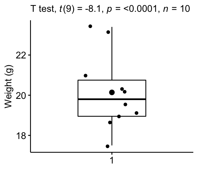
Density plot
Create a density plot with p-value:
- Red line corresponds to the observed mean
- Blue line corresponds to the theoretical mean
ggdensity(mice, x = "weight", rug = TRUE, fill = "lightgray") +
  scale_x_continuous(limits = c(15, 27)) +
  stat_central_tendency(type = "mean", color = "red", linetype = "dashed") +
  geom_vline(xintercept = 25, color = "blue", linetype = "dashed") +
  labs(subtitle = get_test_label(stat.test,  detailed = TRUE))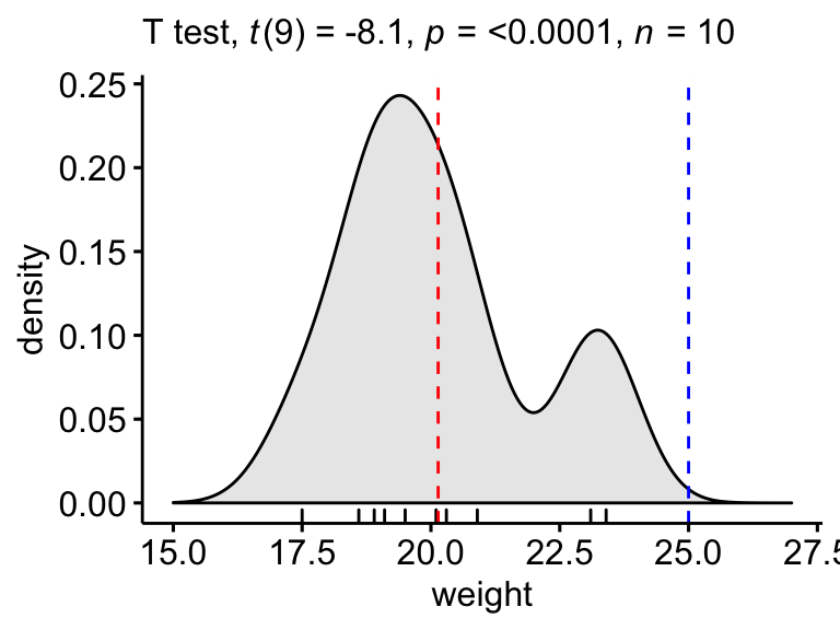
Summary
This article shows how to perform the one-sample t-test in R/Rstudio using two different ways: the R base function t.test() and the t_test() function in the rstatix package. We also describe how to interpret and report the t-test results.
References
Cohen, J. 1998. Statistical Power Analysis for the Behavioral Sciences. 2nd ed. Hillsdale, NJ: Lawrence Erlbaum Associates.
Recommended for you
This section contains best data science and self-development resources to help you on your path.
Books - Data Science
Our Books
- Practical Guide to Cluster Analysis in R by A. Kassambara (Datanovia)
- Practical Guide To Principal Component Methods in R by A. Kassambara (Datanovia)
- Machine Learning Essentials: Practical Guide in R by A. Kassambara (Datanovia)
- R Graphics Essentials for Great Data Visualization by A. Kassambara (Datanovia)
- GGPlot2 Essentials for Great Data Visualization in R by A. Kassambara (Datanovia)
- Network Analysis and Visualization in R by A. Kassambara (Datanovia)
- Practical Statistics in R for Comparing Groups: Numerical Variables by A. Kassambara (Datanovia)
- Inter-Rater Reliability Essentials: Practical Guide in R by A. Kassambara (Datanovia)
Others
- R for Data Science: Import, Tidy, Transform, Visualize, and Model Data by Hadley Wickham & Garrett Grolemund
- Hands-On Machine Learning with Scikit-Learn, Keras, and TensorFlow: Concepts, Tools, and Techniques to Build Intelligent Systems by Aurelien Géron
- Practical Statistics for Data Scientists: 50 Essential Concepts by Peter Bruce & Andrew Bruce
- Hands-On Programming with R: Write Your Own Functions And Simulations by Garrett Grolemund & Hadley Wickham
- An Introduction to Statistical Learning: with Applications in R by Gareth James et al.
- Deep Learning with R by François Chollet & J.J. Allaire
- Deep Learning with Python by François Chollet
Version:
 Français

No Comments