This article describes the t-test assumptions and provides examples of R code to check whether the assumptions are met before calculating the t-test.
You will learn the assumptions of the different types of t-test, including the:
- one-sample t-test
- independent t-test
- paired t-test
Contents:
Related Book
Practical Statistics in R II - Comparing Groups: Numerical VariablesAssumptions
T-test is a parametric test that assumes some characteristics about the data. This section shows the assumptions made by the different t-tests.
- One-sample t-test:
- no significant outliers in the data
- the data should be normally distributed.
- Independent sample t-test:
- no significant outliers in the two groups
- the two groups of samples (A and B), being compared, should be normally distributed.
- the variances of the two groups should not be significantly different. This assumption is made only by the original Student’s t-test. It is relaxed in the Welch’s t-test.
- Paired sample t-test:
- No significant outliers in the difference between the two related groups
- the difference of pairs should follow a normal distribution.
Before using a parametric test, some preliminary tests should be performed to make sure that the test assumptions are met.
In the situations where the assumptions are violated, non-parametric tests, such as Wilcoxon test, are recommended.
Check t-test assumptions in R
Prerequisites
Make sure you have installed the following R packages:
tidyversefor data manipulation and visualizationggpubrfor creating easily publication ready plotsrstatixprovides pipe-friendly R functions for easy statistical analyses.datarium: contains required data sets for this chapter.
Start by loading the following required packages:
library(tidyverse)
library(ggpubr)
library(rstatix)
Check one-sample t-test assumptions
Demo data
Demo dataset: mice [in datarium package]. Contains the weight of 10 mice:
# Load and inspect the data
data(mice, package = "datarium")
head(mice, 3)
## # A tibble: 3 x 2
## name weight
## <chr> <dbl>
## 1 M_1 18.9
## 2 M_2 19.5
## 3 M_3 23.1Identify outliers
Outliers can be easily identified using boxplot methods, implemented in the R function identify_outliers() [rstatix package].
mice %>% identify_outliers(weight)## [1] name weight is.outlier is.extreme
## <0 rows> (or 0-length row.names)There were no extreme outliers.
Note that, in the situation where you have extreme outliers, this can be due to: 1) data entry errors, measurement errors or unusual values.
In this case, you could consider running the non parametric Wilcoxon test.
Check normality assumption
The normality assumption can be checked by computing the Shapiro-Wilk test. If the data is normally distributed, the p-value should be greater than 0.05.
mice %>% shapiro_test(weight)## # A tibble: 1 x 3
## variable statistic p
## <chr> <dbl> <dbl>
## 1 weight 0.923 0.382From the output, the p-value is greater than the significance level 0.05 indicating that the distribution of the data are not significantly different from the normal distribution. In other words, we can assume the normality.
You can also create a QQ plot of the weight data. QQ plot draws the correlation between a given data and the normal distribution.
ggqqplot(mice, x = "weight")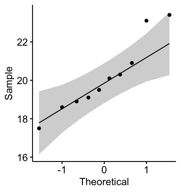
All the points fall approximately along the (45-degree) reference line, for each group. So we can assume normality of the data.
Note that, if your sample size is greater than 50, the normal QQ plot is preferred because at larger sample sizes the Shapiro-Wilk test becomes very sensitive even to a minor deviation from normality.
If the data are not normally distributed, it’s recommended to use a non-parametric test such as the one-sample Wilcoxon signed-rank test. This test is similar to the one-sample t-test, but focuses on the median rather than the mean.
Check independent t-test assumptions
Demo data
Demo dataset: genderweight [in datarium package] containing the weight of 40 individuals (20 women and 20 men).
Load the data and show some random rows by groups:
# Load the data
data("genderweight", package = "datarium")
# Show a sample of the data by group
set.seed(123)
genderweight %>% sample_n_by(group, size = 2)
## # A tibble: 4 x 3
## id group weight
## <fct> <fct> <dbl>
## 1 6 F 65.0
## 2 15 F 65.9
## 3 29 M 88.9
## 4 37 M 77.0Identify outliers by groups
genderweight %>%
  group_by(group) %>%
  identify_outliers(weight)
## # A tibble: 2 x 5
## group id weight is.outlier is.extreme
## <fct> <fct> <dbl> <lgl> <lgl>
## 1 F 20 68.8 TRUE FALSE
## 2 M 31 95.1 TRUE FALSEThere were no extreme outliers.
Check normality by groups
# Compute Shapiro wilk test by goups
data(genderweight, package = "datarium")
genderweight %>%
  group_by(group) %>%
  shapiro_test(weight)
## # A tibble: 2 x 4
## group variable statistic p
## <fct> <chr> <dbl> <dbl>
## 1 F weight 0.938 0.224
## 2 M weight 0.986 0.989# Draw a qq plot by group
ggqqplot(genderweight, x = "weight", facet.by = "group")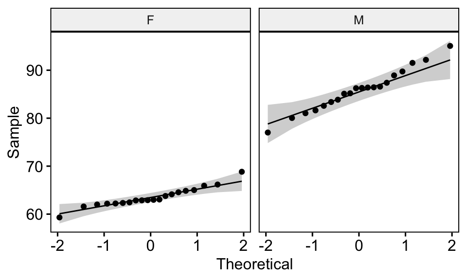
From the output above, we can conclude that the data of the two groups are normally distributed.
Check the equality of variances
This can be done using the Levene’s test. If the variances of groups are equal, the p-value should be greater than 0.05.
genderweight %>% levene_test(weight ~ group)## # A tibble: 1 x 4
## df1 df2 statistic p
## <int> <int> <dbl> <dbl>
## 1 1 38 6.12 0.0180The p-value of the Levene’s test is significant, suggesting that there is a significant difference between the variances of the two groups. Therefore, we’ll use the Welch t-test, which doesn’t assume the equality of the two variances.
Check paired t-test assumptions
Demo data
Here, we’ll use a demo dataset mice2 [datarium package], which contains the weight of 10 mice before and after the treatment.
# Wide format
data("mice2", package = "datarium")
head(mice2, 3)
## id before after
## 1 1 187 430
## 2 2 194 404
## 3 3 232 406# Transform into long data:
# gather the before and after values in the same column
mice2.long <- mice2 %>%
gather(key = "group", value = "weight", before, after)
head(mice2.long, 3)## id group weight
## 1 1 before 187
## 2 2 before 194
## 3 3 before 232First, start by computing the difference between groups:
mice2 <- mice2 %>% mutate(differences = before - after)
head(mice2, 3)
## id before after differences
## 1 1 187 430 -242
## 2 2 194 404 -210
## 3 3 232 406 -174Identify outliers
mice2 %>% identify_outliers(differences)## [1] id before after differences is.outlier is.extreme
## <0 rows> (or 0-length row.names)There were no extreme outliers.
Check normality assumption
# Shapiro-Wilk normality test for the differences
mice2 %>% shapiro_test(differences)
## # A tibble: 1 x 3
## variable statistic p
## <chr> <dbl> <dbl>
## 1 differences 0.968 0.867# QQ plot for the difference
ggqqplot(mice2, "differences")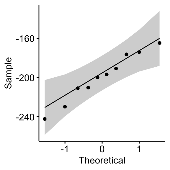
From the output above, it can be assumed that the differences are normally distributed.
Recommended for you
This section contains best data science and self-development resources to help you on your path.
Books - Data Science
Our Books
- Practical Guide to Cluster Analysis in R by A. Kassambara (Datanovia)
- Practical Guide To Principal Component Methods in R by A. Kassambara (Datanovia)
- Machine Learning Essentials: Practical Guide in R by A. Kassambara (Datanovia)
- R Graphics Essentials for Great Data Visualization by A. Kassambara (Datanovia)
- GGPlot2 Essentials for Great Data Visualization in R by A. Kassambara (Datanovia)
- Network Analysis and Visualization in R by A. Kassambara (Datanovia)
- Practical Statistics in R for Comparing Groups: Numerical Variables by A. Kassambara (Datanovia)
- Inter-Rater Reliability Essentials: Practical Guide in R by A. Kassambara (Datanovia)
Others
- R for Data Science: Import, Tidy, Transform, Visualize, and Model Data by Hadley Wickham & Garrett Grolemund
- Hands-On Machine Learning with Scikit-Learn, Keras, and TensorFlow: Concepts, Tools, and Techniques to Build Intelligent Systems by Aurelien Géron
- Practical Statistics for Data Scientists: 50 Essential Concepts by Peter Bruce & Andrew Bruce
- Hands-On Programming with R: Write Your Own Functions And Simulations by Garrett Grolemund & Hadley Wickham
- An Introduction to Statistical Learning: with Applications in R by Gareth James et al.
- Deep Learning with R by François Chollet & J.J. Allaire
- Deep Learning with Python by François Chollet
Version:
 Français

No Comments