This article describes the independent Student T-test, which is used to compare the means of two independent groups. This test is also referred as Students t-test, Student’s t-test and equal variance t-test. For example, you might want to compare the average weights of individuals grouped by gender: male and female groups, which are two unrelated/independent groups.
The independent samples t-test comes in two different forms:
- the standard Student’s t-test, which assumes that the variance of the two groups are equal.
- the Welch’s t-test, which is less restrictive compared to the original Student’s test. This test is described in a dedicated chapter.
Note that, the Welch t-test is considered as the safer one. Usually, the results of the classical student’s t-test and the Welch t-test are very similar unless both the group sizes and the standard deviations are very different.
In this article, you will learn:
- Student t-test formula and assumptions
- How to compute, interpret and report the Student t-test in R.
- How to check the Student t-test assumptions
Contents:
Related Book
Practical Statistics in R II - Comparing Groups: Numerical VariablesPrerequisites
Make sure you have installed the following R packages:
tidyversefor data manipulation and visualizationggpubrfor creating easily publication ready plotsrstatixprovides pipe-friendly R functions for easy statistical analyses.datarium: contains required data sets for this chapter.
Start by loading the following required packages:
library(tidyverse)
library(ggpubr)
library(rstatix)
Research questions
A typical research questions is: whether the mean of group A (\(m_A\)) is equal to the mean of group B (\(m_B\))?
Statistical hypotheses
- Null hypothesis (Ho): the two group means are identical (\(m_A = m_B\))
- Alternative hypothesis (Ha): the two group means are different (\(m_A \ne m_B\))
Formula
The classical Student’s t-test is more restrictive. It assumes that the two groups have the same population variance. If the variance of the two groups are equivalent (homoscedasticity), the t-test value, comparing the two samples (A and B), can be calculated as follow.
\[
t = \frac{m_A - m_B}{\sqrt{ \frac{S^2}{n_A} + \frac{S^2}{n_B} }}
\]
where,
- \(m_A\) and \(m_B\) represent the mean value of the group A and B, respectively.
- \(n_A\) and \(n_B\) represent the sizes of the group A and B, respectively.
- \(S^2\) is an estimator of the pooled variance of the two groups. It can be calculated as follow :
\[
S^2 = \frac{\sum{(x-m_A)^2}+\sum{(x-m_B)^2}}{n_A+n_B-2}
\]
with degrees of freedom (df): \(df = n_A + n_B - 2\).
A p-value can be computed for the corresponding absolute value of t-statistic (|t|).
If the p-value is inferior or equal to the significance level 0.05, we can reject the null hypothesis and accept the alternative hypothesis. In other words, we can conclude that the mean values of group A and B are significantly different.
Assumptions and preleminary tests
The two-samples independent t-test assumes the following characteristics about the data:
- Independence of the observations. Each subject should belong to only one group.
- No significant outliers in the two groups
- Normality. the data for each group should be approximately normally distributed.
- Homogeneity of variances. the variance of the outcome variable should be equal in each group.
Click to check the Student t-test assumptions.
Calculating the test in R
Demo data
Demo dataset: genderweight [in datarium package] containing the weight of 40 individuals (20 women and 20 men).
Load the data and show some random rows by groups:
# Load the data
data("genderweight", package = "datarium")
# Show a sample of the data by group
set.seed(123)
genderweight %>% sample_n_by(group, size = 2)
## # A tibble: 4 x 3
## id group weight
## <fct> <fct> <dbl>
## 1 6 F 65.0
## 2 15 F 65.9
## 3 29 M 88.9
## 4 37 M 77.0Summary statistics
Compute some summary statistics by groups: mean and sd (standard deviation)
genderweight %>%
  group_by(group) %>%
  get_summary_stats(weight, type = "mean_sd")
## # A tibble: 2 x 5
## group variable n mean sd
## <fct> <chr> <dbl> <dbl> <dbl>
## 1 F weight 20 63.5 2.03
## 2 M weight 20 85.8 4.35Visualization
Visualize the data using box plots. Plot weight by groups.
bxp <- ggboxplot(
  genderweight, x = "group", y = "weight",
  ylab = "Weight", xlab = "Groups", add = "jitter"
  )
bxp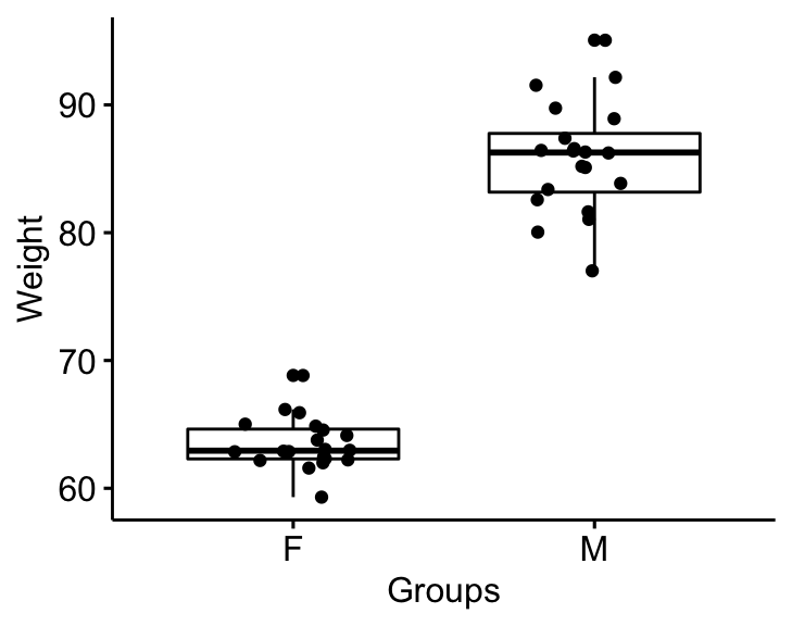
Computation
We’ll use the pipe-friendly t_test() function [rstatix package], a wrapper around the R base function t.test().
Recall that, by default, R computes the Welch t-test, which is the safer one. This is the test where you do not assume that the variance is the same in the two groups, which results in the fractional degrees of freedom. If you want to assume the equality of variances (Student t-test), specify the option var.equal = TRUE:
stat.test <- genderweight %>%
  t_test(weight ~ group, var.equal = TRUE) %>%
  add_significance()
stat.test
## # A tibble: 1 x 9
## .y. group1 group2 n1 n2 statistic df p p.signif
## <chr> <chr> <chr> <int> <int> <dbl> <dbl> <dbl> <chr>
## 1 weight F M 20 20 -20.8 38 2.33e-22 ****The results above show the following components:
.y.: the y variable used in the test.group1,group2: the compared groups in the pairwise tests.statistic: Test statistic used to compute the p-value.df: degrees of freedom.p: p-value.
Note that, you can obtain a detailed result by specifying the option detailed = TRUE.
Cohen’s d for Student t-test
This effect size is calculated by dividing the mean difference between the groups by the pooled standard deviation.
Cohen’s d formula:
d = (mean1 - mean2)/pooled.sd, where:
pooled.sdis the common standard deviation of the two groups.pooled.sd = sqrt([var1*(n1-1) + var2*(n2-1)]/[n1 + n2 -2]);var1andvar2are the variances (squared standard deviation) of group1 and 2, respectively.n1andn2are the sample counts for group 1 and 2, respectively.mean1andmean2are the means of each group, respectively.
Calculation:
genderweight %>% cohens_d(weight ~ group, var.equal = TRUE)## # A tibble: 1 x 7
## .y. group1 group2 effsize n1 n2 magnitude
## * <chr> <chr> <chr> <dbl> <int> <int> <ord>
## 1 weight F M -6.57 20 20 largeThere is a large effect size, d = 6.57.
Report
We could report the result as follow:
The mean weight in female group was 63.5 (SD = 2.03), whereas the mean in male group was 85.8 (SD = 4.3). A Student t-test showed that the difference was statistically significant, t(38) = -20.8, p < 0.0001, d = 6.57; where, t(38) is shorthand notation for a Student t-statistic that has 38 degrees of freedom.
stat.test <- stat.test %>% add_xy_position(x = "group")
bxp +
  stat_pvalue_manual(stat.test, tip.length = 0) +
  labs(subtitle = get_test_label(stat.test, detailed = TRUE))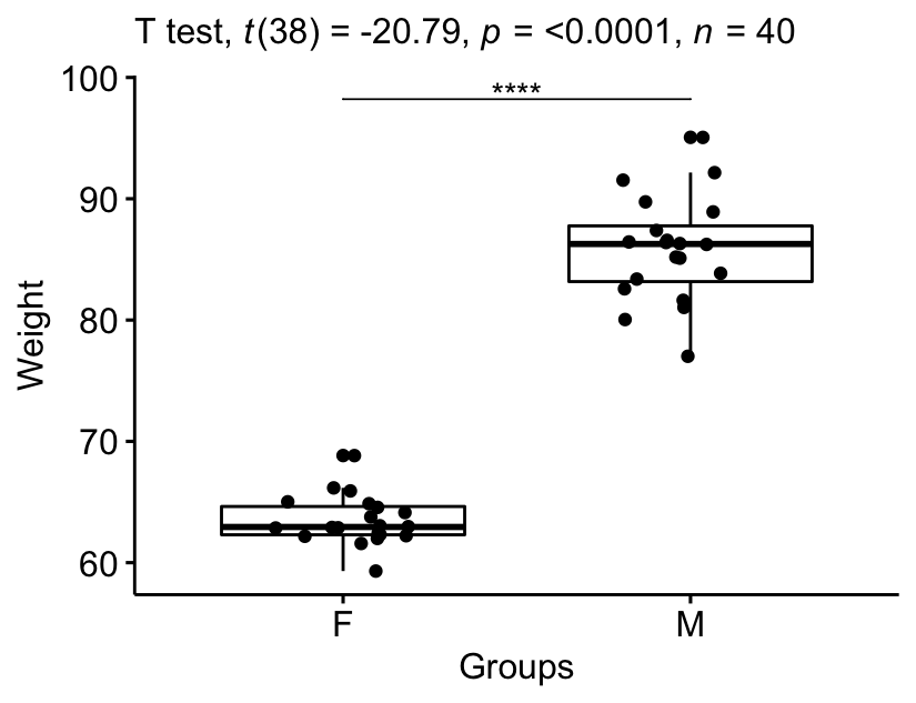
Summary
This article describes the formula and the basics of the Student t-test. Examples of R codes are provided for computing the test and the effect size, interpreting and reporting the results.
Recommended for you
This section contains best data science and self-development resources to help you on your path.
Books - Data Science
Our Books
- Practical Guide to Cluster Analysis in R by A. Kassambara (Datanovia)
- Practical Guide To Principal Component Methods in R by A. Kassambara (Datanovia)
- Machine Learning Essentials: Practical Guide in R by A. Kassambara (Datanovia)
- R Graphics Essentials for Great Data Visualization by A. Kassambara (Datanovia)
- GGPlot2 Essentials for Great Data Visualization in R by A. Kassambara (Datanovia)
- Network Analysis and Visualization in R by A. Kassambara (Datanovia)
- Practical Statistics in R for Comparing Groups: Numerical Variables by A. Kassambara (Datanovia)
- Inter-Rater Reliability Essentials: Practical Guide in R by A. Kassambara (Datanovia)
Others
- R for Data Science: Import, Tidy, Transform, Visualize, and Model Data by Hadley Wickham & Garrett Grolemund
- Hands-On Machine Learning with Scikit-Learn, Keras, and TensorFlow: Concepts, Tools, and Techniques to Build Intelligent Systems by Aurelien Géron
- Practical Statistics for Data Scientists: 50 Essential Concepts by Peter Bruce & Andrew Bruce
- Hands-On Programming with R: Write Your Own Functions And Simulations by Garrett Grolemund & Hadley Wickham
- An Introduction to Statistical Learning: with Applications in R by Gareth James et al.
- Deep Learning with R by François Chollet & J.J. Allaire
- Deep Learning with Python by François Chollet
Version:
 Français

No Comments