The unpaired t-test is used to compare the mean of two independent groups. It’s also known as:
- independent samples t-test,
- independent t-test,
- 2 sample t test,
- two sample t-test,
- independent-measures t-test,
- independent groups t test,
- unpaired student t test,
- between-subjects t-test and
- Student’s t-test.
For example, you might want to compare the average weights of individuals grouped by gender: male and female groups, which are two unrelated/independent groups.
As a rule of thumb, your study should have six or more participants in each group in order to proceed with an unpaired t-test, but ideally you would have more. An independent-samples t-test will run with less than six participants, but your ability to generalize to a larger population will be more difficult.
The independent samples t-test comes in two different forms:
- the standard Student’s t-test, which assumes that the variance of the two groups are equal.
- the Welch’s t-test, which is less restrictive compared to the original Student’s test. This is the test where you do not assume that the variance is the same in the two groups, which results in the fractional degrees of freedom.
By default, R computes the Welch t-test, which is the safer one. The two methods give very similar results unless both the group sizes and the standard deviations are very different.
In this article, you will learn how to:
- Compute the independent samples t-test in R. The pipe-friendly function
t_test()[rstatix package] will be used. - Check the independent-samples t-test assumptions
- Calculate and report the independent samples t-test effect size using Cohen’s d. The
dstatistic redefines the difference in means as the number of standard deviations that separates those means. T-test conventional effect sizes, proposed by Cohen, are: 0.2 (small effect), 0.5 (moderate effect) and 0.8 (large effect) (Cohen 1998).
Contents:
Related Book
Practical Statistics in R II - Comparing Groups: Numerical VariablesPrerequisites
Make sure you have installed the following R packages:
tidyversefor data manipulation and visualizationggpubrfor creating easily publication ready plotsrstatixprovides pipe-friendly R functions for easy statistical analyses.datarium: contains required data sets for this chapter.
Start by loading the following required packages:
library(tidyverse)
library(ggpubr)
library(rstatix)
Research questions
Typical research questions are:
- whether the mean of group A (\(m_A\)) is equal to the mean of group B (\(m_B\))?
- whether the mean of group A (\(m_A\)) is less than the mean of group B (\(m_B\))?
- whether the mean of group A (\(m_A\)) is greater than the mean of group B (\(m_B\))?
Statistical hypotheses
In statistics, we can define the corresponding null hypothesis (\(H_0\)) as follow:
- \(H_0: m_A = m_B\)
- \(H_0: m_A \leq m_B\)
- \(H_0: m_A \geq m_B\)
The corresponding alternative hypotheses (\(H_a\)) are as follow:
- \(H_a: m_A \ne m_B\) (different)
- \(H_a: m_A > m_B\) (greater)
- \(H_a: m_A < m_B\) (less)
Note that:
- Hypotheses 1) are called two-tailed tests
- Hypotheses 2) and 3) are called one-tailed tests
Formula
The independent samples t-test comes in two different forms, Student’s t-test and Welch’s t-test.
The classical Student’s t-test is more restrictive. It assumes that the two groups have the same population variance.
- Classical two independent samples t-test (Student t-test). If the variance of the two groups are equivalent (homoscedasticity), the t-test value, comparing the two samples (A and B), can be calculated as follow.
\[
t = \frac{m_A - m_B}{\sqrt{ \frac{S^2}{n_A} + \frac{S^2}{n_B} }}
\]
where,
- \(m_A\) and \(m_B\) represent the mean value of the group A and B, respectively.
- \(n_A\) and \(n_B\) represent the sizes of the group A and B, respectively.
- \(S^2\) is an estimator of the pooled variance of the two groups. It can be calculated as follow :
\[
S^2 = \frac{\sum{(x-m_A)^2}+\sum{(x-m_B)^2}}{n_A+n_B-2}
\]
with degrees of freedom (df): \(df = n_A + n_B - 2\).
- Welch t-statistic. If the variances of the two groups being compared are different (heteroscedasticity), it’s possible to use the Welch t-test, which is an adaptation of the Student t-test. The Welch t-statistic is calculated as follow :
\[
t = \frac{m_A - m_B}{\sqrt{ \frac{S_A^2}{n_A} + \frac{S_B^2}{n_B} }}
\]
where, \(S_A\) and \(S_B\) are the standard deviation of the the two groups A and B, respectively.
Unlike the classic Student’s t-test, the Welch t-test formula involves the variance of each of the two groups (\(S_A^2\) and \(S_B^2\)) being compared. In other words, it does not use the pooled variance \(S\).
The degrees of freedom of Welch t-test is estimated as follow :
\[
df = (\frac{S_A^2}{n_A}+ \frac{S_B^2}{n_B})^2 / (\frac{S_A^4}{n_A^2(n_A-1)} + \frac{S_B^4}{n_B^2(n_B-1)} )
\]
A p-value can be computed for the corresponding absolute value of t-statistic (|t|).
If the p-value is inferior or equal to the significance level 0.05, we can reject the null hypothesis and accept the alternative hypothesis. In other words, we can conclude that the mean values of group A and B are significantly different.
Note that, the Welch t-test is considered as the safer one. Usually, the results of the classical student’s t-test and the Welch t-test are very similar unless both the group sizes and the standard deviations are very different.
Demo data
Demo dataset: genderweight [in datarium package] containing the weight of 40 individuals (20 women and 20 men).
Load the data and show some random rows by groups:
# Load the data
data("genderweight", package = "datarium")
# Show a sample of the data by group
set.seed(123)
genderweight %>% sample_n_by(group, size = 2)
## # A tibble: 4 x 3
## id group weight
## <fct> <fct> <dbl>
## 1 6 F 65.0
## 2 15 F 65.9
## 3 29 M 88.9
## 4 37 M 77.0Summary statistics
Compute some summary statistics by groups: mean and sd (standard deviation)
genderweight %>%
  group_by(group) %>%
  get_summary_stats(weight, type = "mean_sd")
## # A tibble: 2 x 5
## group variable n mean sd
## <fct> <chr> <dbl> <dbl> <dbl>
## 1 F weight 20 63.5 2.03
## 2 M weight 20 85.8 4.35Visualization
Visualize the data using box plots. Plot weight by groups.
bxp <- ggboxplot(
  genderweight, x = "group", y = "weight",
  ylab = "Weight", xlab = "Groups", add = "jitter"
  )
bxp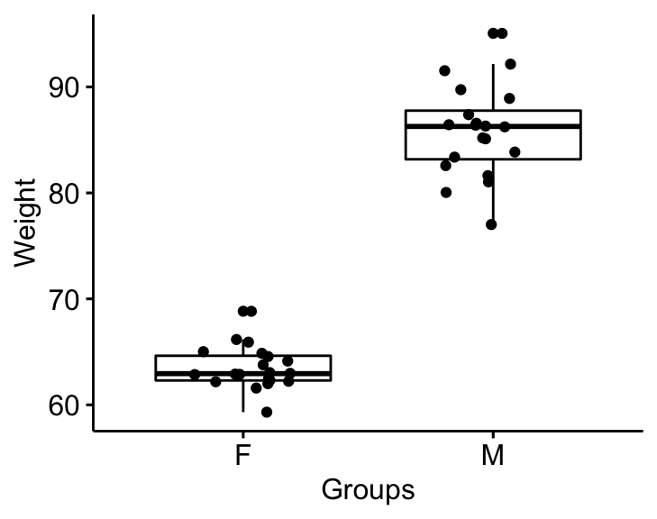
Assumptions and preleminary tests
The two-samples independent t-test assume the following characteristics about the data:
- Independence of the observations. Each subject should belong to only one group. There is no relationship between the observations in each group.
- No significant outliers in the two groups
- Normality. the data for each group should be approximately normally distributed.
- Homogeneity of variances. the variance of the outcome variable should be equal in each group.
In this section, we’ll perform some preliminary tests to check whether these assumptions are met.
Identify outliers
Outliers can be easily identified using boxplot methods, implemented in the R function identify_outliers() [rstatix package].
genderweight %>%
  group_by(group) %>%
  identify_outliers(weight)
## # A tibble: 2 x 5
## group id weight is.outlier is.extreme
## <fct> <fct> <dbl> <lgl> <lgl>
## 1 F 20 68.8 TRUE FALSE
## 2 M 31 95.1 TRUE FALSEThere were no extreme outliers.
Note that, in the situation where you have extreme outliers, this can be due to: 1) data entry errors, measurement errors or unusual values.
Yo can include the outlier in the analysis anyway if you do not believe the result will be substantially affected. This can be evaluated by comparing the result of the t-test with and without the outlier.
It’s also possible to keep the outliers in the data and perform Wilcoxon test or robust t-test using the WRS2 package.
Check normality by groups
The normality assumption can be checked by computing the Shapiro-Wilk test for each group. If the data is normally distributed, the p-value should be greater than 0.05.
genderweight %>%
  group_by(group) %>%
  shapiro_test(weight)
## # A tibble: 2 x 4
## group variable statistic p
## <fct> <chr> <dbl> <dbl>
## 1 F weight 0.938 0.224
## 2 M weight 0.986 0.989From the output, the two p-values are greater than the significance level 0.05 indicating that the distribution of the data are not significantly different from the normal distribution. In other words, we can assume the normality.
You can also create QQ plots for each group. QQ plot draws the correlation between a given data and the normal distribution.
ggqqplot(genderweight, x = "weight", facet.by = "group")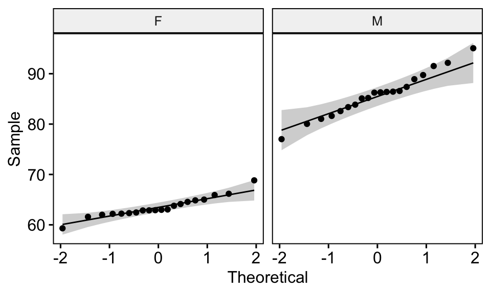
All the points fall approximately along the (45-degree) reference line, for each group. So we can assume normality of the data.
Note that, if your sample size is greater than 50, the normal QQ plot is preferred because at larger sample sizes the Shapiro-Wilk test becomes very sensitive even to a minor deviation from normality.
Note that, in the situation where the data are not normally distributed, it’s recommended to use the non parametric two-samples Wilcoxon test.
Check the equality of variances
This can be done using the Levene’s test. If the variances of groups are equal, the p-value should be greater than 0.05.
genderweight %>% levene_test(weight ~ group)## # A tibble: 1 x 4
## df1 df2 statistic p
## <int> <int> <dbl> <dbl>
## 1 1 38 6.12 0.0180The p-value of the Levene’s test is significant, suggesting that there is a significant difference between the variances of the two groups. Therefore, we’ll use the Welch t-test, which doesn’t assume the equality of the two variances.
Computation
We want to know, whether the average weights are different between groups.
We’ll use the pipe-friendly t_test() function [rstatix package], a wrapper around the R base function t.test().
Recall that, by default, R computes the Welch t-test, which is the safer one. This is the test where you do not assume that the variance is the same in the two groups, which results in the fractional degrees of freedom.
stat.test <- genderweight %>%
  t_test(weight ~ group) %>%
  add_significance()
stat.test
## # A tibble: 1 x 9
## .y. group1 group2 n1 n2 statistic df p p.signif
## <chr> <chr> <chr> <int> <int> <dbl> <dbl> <dbl> <chr>
## 1 weight F M 20 20 -20.8 26.9 4.30e-18 ****If you want to assume the equality of variances (Student t-test), specify the option var.equal = TRUE:
stat.test2 <- genderweight %>%
  t_test(weight ~ group, var.equal = TRUE) %>%
  add_significance()
stat.test2
The results above show the following components:
.y.: the y variable used in the test.group1,group2: the compared groups in the pairwise tests.statistic: Test statistic used to compute the p-value.df: degrees of freedom.p: p-value.
Note that, you can obtain a detailed result by specifying the option detailed = TRUE.
Note that, to compute one tailed two samples t-test, you can specify the option alternative as follow.
- if you want to test whether the average women’s weight (group 1) is less than the average men’s weight (group 2), type this:
genderweight %>%
t_test(weight ~ group, alternative = "less")- Or, if you want to test whether the average women’s weight (group 1) is greater than the average men’s weight (group 2), type this
genderweight %>%
  t_test(weight ~ group, alternative = "greater")
Effect size
Cohen’s d for Student t-test
There are multiple version of Cohen’s d for Student t-test. The most commonly used version of the Student t-test effect size, comparing two groups (A and B), is calculated by dividing the mean difference between the groups by the pooled standard deviation.
Cohen’s d formula:
\[
d = \frac{m_A - m_B}{SD_{pooled}}
\]
where,
- \(m_A\) and \(m_B\) represent the mean value of the group A and B, respectively.
- \(n_A\) and \(n_B\) represent the sizes of the group A and B, respectively.
- \(SD_{pooled}\) is an estimator of the pooled standard deviation of the two groups. It can be calculated as follow :
\[
SD_{pooled} = \sqrt{\frac{\sum{(x-m_A)^2}+\sum{(x-m_B)^2}}{n_A+n_B-2}}
\]
Calculation. If the option var.equal = TRUE, then the pooled SD is used when computing the Cohen’s d.
genderweight %>% cohens_d(weight ~ group, var.equal = TRUE)## # A tibble: 1 x 7
## .y. group1 group2 effsize n1 n2 magnitude
## * <chr> <chr> <chr> <dbl> <int> <int> <ord>
## 1 weight F M -6.57 20 20 largeThere is a large effect size, d = 6.57.
Note that, for small sample size (< 50), the Cohen’s d tends to over-inflate results. There exists a Hedge’s Corrected version of the Cohen’s d (Hedges and Olkin 1985), which reduces effect sizes for small samples by a few percentage points. The correction is introduced by multiplying the usual value of d by (N-3)/(N-2.25) (for unpaired t-test) and by (n1-2)/(n1-1.25) for paired t-test; where N is the total size of the two groups being compared (N = n1 + n2).
Cohen’s d for Welch t-test
The Welch test is a variant of t-test used when the equality of variance can’t be assumed. The effect size can be computed by dividing the mean difference between the groups by the “averaged” standard deviation.
Cohen’s d formula:
\[
d = \frac{m_A - m_B}{\sqrt{(Var_1 + Var_2)/2}}
\]
where,
- \(m_A\) and \(m_B\) represent the mean value of the group A and B, respectively.
- \(Var_1\) and \(Var_2\) are the variance of the two groups.
Calculation:
genderweight %>% cohens_d(weight ~ group, var.equal = FALSE)## # A tibble: 1 x 7
## .y. group1 group2 effsize n1 n2 magnitude
## * <chr> <chr> <chr> <dbl> <int> <int> <ord>
## 1 weight F M -6.57 20 20 largeNote that, when group sizes are equal and group variances are homogeneous, Cohen’s d for the standard Student and Welch t-tests are identical.
Report
We could report the result as follow:
The mean weight in female group was 63.5 (SD = 2.03), whereas the mean in male group was 85.8 (SD = 4.3). A Welch two-samples t-test showed that the difference was statistically significant, t(26.9) = -20.8, p < 0.0001, d = 6.57; where, t(26.9) is shorthand notation for a Welch t-statistic that has 26.9 degrees of freedom.
stat.test <- stat.test %>% add_xy_position(x = "group")
bxp +
  stat_pvalue_manual(stat.test, tip.length = 0) +
  labs(subtitle = get_test_label(stat.test, detailed = TRUE))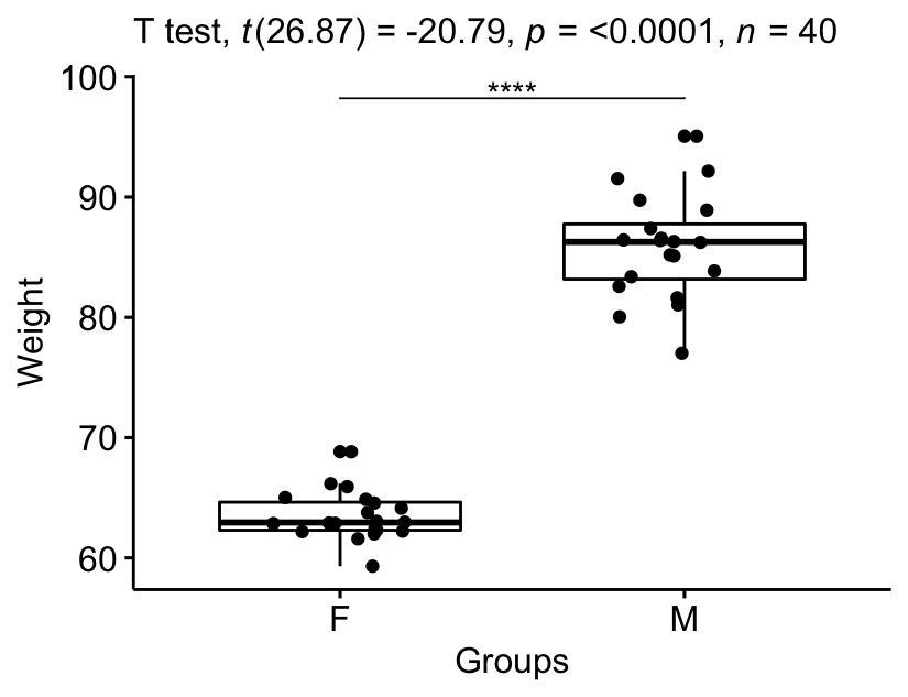
Summary
This article describes the formula and the basics of the unpaired t-test or independent t-test. Examples of R codes are provided to check the assumptions, computing the test and the effect size, interpreting and reporting the results.
References
Cohen, J. 1998. Statistical Power Analysis for the Behavioral Sciences. 2nd ed. Hillsdale, NJ: Lawrence Erlbaum Associates.
Hedges, Larry, and Ingram Olkin. 1985. “Statistical Methods in Meta-Analysis.” In Stat Med. Vol. 20. doi:10.2307/1164953.
Recommended for you
This section contains best data science and self-development resources to help you on your path.
Books - Data Science
Our Books
- Practical Guide to Cluster Analysis in R by A. Kassambara (Datanovia)
- Practical Guide To Principal Component Methods in R by A. Kassambara (Datanovia)
- Machine Learning Essentials: Practical Guide in R by A. Kassambara (Datanovia)
- R Graphics Essentials for Great Data Visualization by A. Kassambara (Datanovia)
- GGPlot2 Essentials for Great Data Visualization in R by A. Kassambara (Datanovia)
- Network Analysis and Visualization in R by A. Kassambara (Datanovia)
- Practical Statistics in R for Comparing Groups: Numerical Variables by A. Kassambara (Datanovia)
- Inter-Rater Reliability Essentials: Practical Guide in R by A. Kassambara (Datanovia)
Others
- R for Data Science: Import, Tidy, Transform, Visualize, and Model Data by Hadley Wickham & Garrett Grolemund
- Hands-On Machine Learning with Scikit-Learn, Keras, and TensorFlow: Concepts, Tools, and Techniques to Build Intelligent Systems by Aurelien Géron
- Practical Statistics for Data Scientists: 50 Essential Concepts by Peter Bruce & Andrew Bruce
- Hands-On Programming with R: Write Your Own Functions And Simulations by Garrett Grolemund & Hadley Wickham
- An Introduction to Statistical Learning: with Applications in R by Gareth James et al.
- Deep Learning with R by François Chollet & J.J. Allaire
- Deep Learning with Python by François Chollet
Version:
 Français

Great lesson overall!
Just one thing I noticed. When you explain the one-tailed variants of the t-tests you say:
“If you want to test whether the average men’s weight is less than the average women’s weight, type this: [alternative = “less”]”
AND
“Or, if you want to test whether the average men’s weight is greater than the average women’s weight, type this: [alternative = “greater”]”
In the example the women’s weight is less than the men’s weight. I get the former one-tailed t-test as significant while the latter is not significant. Isn’t there a mistake in the description?
At least on my system, “alternative = “less”” examines whether the average women’s weight is less than the average men’s weight, and vice versa. Am I understanding it correctly?
Thank you for pointing this out, updated now! Correct sentences are:
1) “if you want to test whether the average women’s weight (group 1) is less than the average men’s weight (group 2), type this : [alternative = “less”]
2) “Or, if you want to test whether the average women’s weight (group 1) is greater than the average men’s weight (group 2), type this”: [alternative = “greater”]