Gene Set Enrichment & Pathway Analysis in R with clusterProfiler
Turn a list of differentially expressed genes into the biological pathways behind it — over-representation analysis and GSEA, interpreted and visualized
Bioinformatics
A practical guide to functional enrichment analysis in R with clusterProfiler. Take a DESeq2 differential expression result and find the biological pathways behind it two ways: over-representation analysis (ORA) on your significant gene shortlist with enrichGO, and gene set enrichment analysis (GSEA) on the full ranked gene list with gseGO. Understand when to use which, read the GeneRatio, NES, and adjusted p-values in plain language, and visualize the result with dot plots and the GSEA running-score plot. On the airway dataset.
Published
June 29, 2026
Modified
July 7, 2026
TipKey takeaways
After differential expression you have hundreds of genes — too many to read one by one. Enrichment analysis asks the better question: which biological pathways shifted as a group?
Two complementary methods.ORA (over-representation analysis) tests whether your significant gene shortlist is unusually full of a pathway’s genes. GSEA (gene set enrichment analysis) uses all genes, ranked, and asks whether a pathway’s genes cluster at the top or bottom.
ORA needs a cutoff (your padj < 0.05 list) and gives no direction; GSEA needs no cutoff and gives a signed score (NES) — up or down. Agreement between them makes a result convincing.
clusterProfiler runs both against many databases. This lesson covers GO Biological Process, MSigDB Hallmark, and Reactome — all from local annotation, so the whole analysis is reproducible offline (KEGG is the one exception — it needs a web API).
Read GeneRatio + p.adjust for ORA, NES (sign = direction) + p.adjust for GSEA, and visualize with a dot plot and the GSEA running-score plot.
Introduction
Differential expression (the DESeq2 lesson) leaves you with a long list of significant genes. Scanning it gene by gene is hopeless and misses the point: biology happens in pathways, not single genes. Enrichment analysis turns the gene list into a much shorter list of biological programmes — immune response, cell cycle, extracellular-matrix organization — that moved together.
There are two standard strategies, and they answer slightly different questions, so it is worth running both. This guide uses clusterProfiler, the standard R toolkit for both, on the differentially expressed genes from the airway experiment (dexamethasone-treated vs untreated airway smooth-muscle cells).
Start from a DESeq2 result
Enrichment takes a differential-expression result as input. We rebuild it here so the lesson stands alone — this is the same workflow as the DESeq2 lesson, condensed.
sum(res$padj <0.05, na.rm =TRUE) # significant at 5% FDR
[1] 4000
About four thousand genes are significant — far too many to interpret directly. That is exactly what enrichment analysis is for.
ORA vs GSEA — two ways to ask the question
The two methods take different inputs and answer different questions. Run both: agreement between them (and across databases) is what makes an enrichment result trustworthy.
ORA (over-representation)
GSEA (gene set enrichment)
Input
your shortlist of significant genes (a yes/no list)
all genes, ranked by a statistic
Question
Is a pathway over-represented in my hit list, more than chance?
Do a pathway’s genes cluster at the top or bottom of the ranking?
Cutoff
needs one (padj / fold-change gate)
none — uses every gene
Direction
no (just “enriched”)
yes — a signed score (up or down)
Best at
a strong, clear-cut hit list
coordinated small shifts of many genes together
In short: ORA asks “is this pathway in my hit list?”; GSEA asks “does this pathway move coherently across the whole experiment, even through many small changes?”
NoteHow they are computed (optional maths)
ORA uses a hypergeometric test (equivalently Fisher’s exact test). With a universe of \(N\) genes, \(K\) in the pathway, \(n\) genes in your shortlist and \(k\) of those in the pathway, the p-value is the chance of seeing at least\(k\) overlaps by chance: \[P(X \ge k) = \sum_{i=k}^{\min(n,K)} \frac{\binom{K}{i}\binom{N-K}{n-i}}{\binom{N}{n}}\]
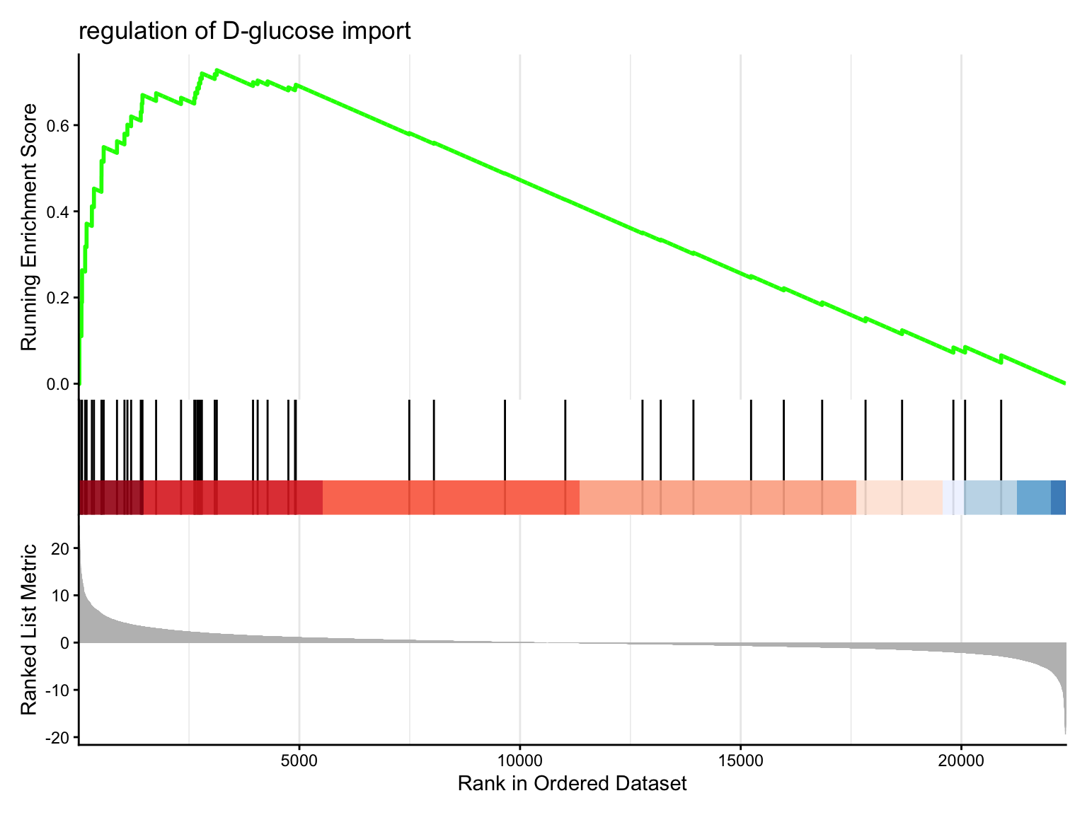
GSEA walks down the ranked gene list keeping a running enrichment score: it steps up at every pathway member (weighted by the gene’s ranking metric) and down at every non-member. The enrichment score (ES) is the furthest that running score gets from zero; the NES normalizes it for gene-set size so sets are comparable, and its sign gives the direction. Significance comes from permuting gene labels many times. Both methods then apply Benjamini–Hochberg correction across all gene sets tested.
Over-representation analysis (ORA)
ORA tests your significant shortlist against every GO term. Two inputs: the gene list (significant genes) and the universe (all genes you tested) — the universe matters, because “enriched” means “more than expected given what could have been detected.”
                                             Description GeneRatio     p.adjust
GO:0001525                                  angiogenesis  197/3382 8.082764e-13
GO:0030198             extracellular matrix organization  130/3382 1.859404e-10
GO:0043062          extracellular structure organization  130/3382 1.859404e-10
GO:0045229 external encapsulating structure organization  130/3382 1.917404e-10
GO:0003013                    circulatory system process  191/3382 3.429143e-10
GO:0003012                         muscle system process  148/3382 7.098788e-10
GO:0030335         positive regulation of cell migration  188/3382 1.318132e-09
GO:2000147          positive regulation of cell motility  192/3382 3.025832e-09
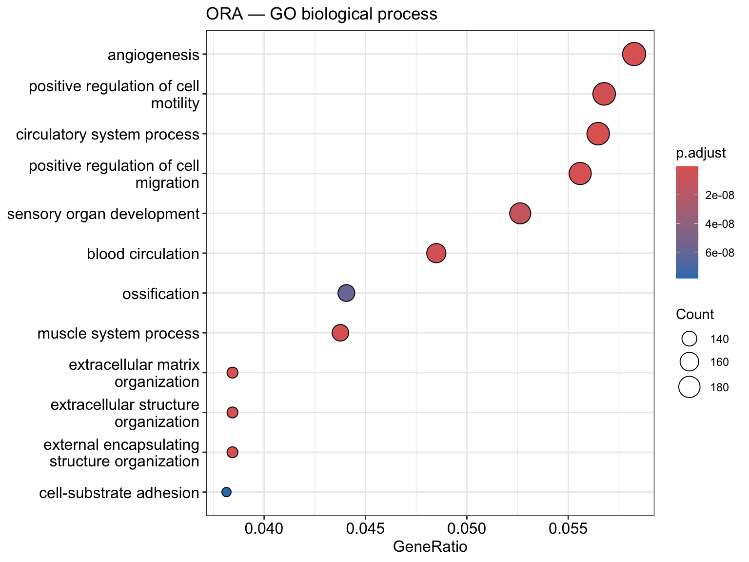
Read the result: GeneRatio is the fraction of your annotated significant genes that fall in the term; p.adjust is its FDR-corrected significance. The enriched terms are tissue-remodelling and vascular programmes — angiogenesis, cell motility and migration, circulatory- and muscle-system processes, and extracellular-matrix organization — coherent biology for glucocorticoid-treated airway smooth muscle, not a random list. That coherence is the sanity check.
Visualize ORA — the dot plot
The dot plot is the standard enrichment figure: one row per term, gene ratio on the x-axis, dot size = the number of genes, colour = adjusted p-value.
library(enrichplot)dotplot(ego, showCategory =12) + ggplot2::ggtitle("ORA — GO biological process")
Gene-concept network — which genes drive which terms
The dot plot shows which terms are enriched; a gene-concept network shows the genes behind them and which terms they share — useful for spotting a handful of genes that drive several pathways at once.
cnetplot(ego, showCategory =5)
Gene set enrichment analysis (GSEA)
GSEA needs no cutoff. Instead of a shortlist, you give it every gene, ranked by a statistic — here the DESeq2 Wald stat, which carries both the direction and the strength of the change. GSEA then asks whether each pathway’s genes drift to the top (up) or bottom (down) of that ranking.
                                               Description       NES
GO:0046324                  regulation of D-glucose import  2.217309
GO:0046323                                D-glucose import  2.208967
GO:0031069                     hair follicle morphogenesis -2.179956
GO:0048730                         epidermis morphogenesis -2.166981
GO:0010827 regulation of D-glucose transmembrane transport  2.103370
GO:1904659               D-glucose transmembrane transport  2.099115
GO:0008645                  hexose transmembrane transport  2.083159
GO:0003382                   epithelial cell morphogenesis  2.066909
               p.adjust
GO:0046324 0.0005072619
GO:0046323 0.0001754471
GO:0031069 0.0010079837
GO:0048730 0.0012691972
GO:0010827 0.0009582575
GO:1904659 0.0005990325
GO:0008645 0.0005072619
GO:0003382 0.0032992484
Read the NES (normalized enrichment score): its magnitude is the strength, its sign the direction — positive = up in treated cells, negative = down. The strongest moves are metabolic and transport programmes shifting up (glucose import/transport) against epidermal and hair-follicle morphogenesis programmes shifting down — a signed, coherent picture that the cutoff-based ORA cannot give you.
Visualize GSEA — the running-score plot
The signature GSEA figure shows the running enrichment score as you walk down the ranked list, with the pathway’s genes marked as ticks. A peak near the top = a pathway enriched among up-regulated genes.
top_id <- gdf$ID[which.max(gdf$NES)] # the most up-regulated setgseaplot2(gse, geneSetID = top_id, title = gdf$Description[gdf$ID == top_id])
Beyond GO — Hallmark and Reactome collections
GO is one vocabulary, rarely the only one you want. Two curated collections give complementary views of the same ranked list, and both run from local annotation packages — no web API — so they stay reproducible:
MSigDB Hallmark — 50 deliberately coarse gene sets, each a well-defined biological programme: the “what shifted, in broad strokes” view.
Reactome — thousands of detailed, clinically-named pathways (signalling cascades, metabolism): the “name it the way a biologist would” view.
Running GSEA on them is the same ranked-list machinery as gseGO — only the gene-set source changes.
Hallmark pathways (GSEA)
Hallmark sets are keyed by gene symbol, so we relabel the ranked list from Ensembl IDs to symbols, then hand it to the generic GSEA() with Hallmark as the gene-set table.
About thirty Hallmark sets clear FDR < 0.25. The strongest, most significant moves are metabolic and signalling programmes shifting up — HALLMARK_ADIPOGENESIS, HALLMARK_TNFA_SIGNALING_VIA_NFKB, HALLMARK_ANDROGEN_RESPONSE, HALLMARK_OXIDATIVE_PHOSPHORYLATION — alongside HALLMARK_P53_PATHWAY moving down (negative NES). That fits the biology: dexamethasone is a glucocorticoid, and a coarse 50-set overview should surface exactly these metabolic and anti-inflammatory signatures.
A dot plot shows the same result at a glance, split by direction:
The dot plot splits the sets by direction — activated (positive NES, up in treated cells) on one side, suppressed on the other — with dot size the leading-edge gene count and colour the adjusted p-value. Reading the two panels side by side is the fastest way to see which programmes went up and which came down.
Reactome pathways (GSEA)
Reactome is indexed by Entrez IDs, so we relabel the ranked list once more, then run GSEA over Reactome pathways with gsePathway().
Reactome’s pathways are finer-grained, so it returns many more hits — here nearly two hundred at FDR < 0.25. The leading pathways are clinically legible and biologically on-point for airway smooth-muscle cells: muscle and smooth-muscle contraction, signal transduction, and neutrophil degranulation moving up, against cytosolic tRNA aminoacylation moving down. This is the level of detail you would cite in a paper’s results.
The same split dot plot, now over Reactome pathways — activated versus suppressed, side by side:
A coarse collection can place an unrelated programme near the top by chance, and no single pathway is ever the whole story. Trust the result that shows up consistently — across GO, Hallmark, and Reactome, and in the direction the biology predicts. Three vocabularies agreeing is what makes an enrichment result convincing.
Common issues
ORA finds nothing, GSEA finds plenty (or vice-versa). They answer different questions, so this is normal. ORA needs a strong, clear-cut shortlist; GSEA detects coordinated small shifts that never pass a per-gene cutoff. Disagreement is information, not a bug — report both.
“No gene can be mapped” / empty result. The keyType must match your gene IDs. airway uses Ensembl IDs, so keyType = "ENSEMBL". If your genes are symbols use "SYMBOL", if Entrez use "ENTREZID" — or convert first with bitr().
You forgot the universe in ORA. Without universe = (all tested genes), enrichGO compares against the whole genome, inflating significance. Always pass the genes that could have been detected in your experiment.
Frequently asked questions
NoteWhat is the difference between ORA and GSEA?
ORA tests a shortlist of significant genes (a yes/no cutoff) for over-representation of a pathway using a hypergeometric test — no direction. GSEA uses all genes ranked by a statistic and asks whether a pathway clusters at the top or bottom, giving a signed NES (up or down) and no need for a cutoff. Use both; agreement is convincing.
NoteHow do I do KEGG pathway analysis in R?
This lesson already runs Reactome (gsePathway) and MSigDB Hallmark (GSEA + msigdbr) above — both from local annotation, fully offline. KEGG is the same workflow (enrichKEGG() / gseKEGG()) with one catch: the KEGG functions need Entrez IDs (convert with bitr()) and query the KEGG web API at runtime, so they require an internet connection — which is why this offline-reproducible lesson doesn’t run a live KEGG cell. For ORA on a shortlist, ReactomePA::enrichPathway() is the over-representation counterpart to the GSEA gsePathway() shown above.
NoteWhich gene ID type should I use?
Match keyType to your data. DESeq2 on airway gives Ensembl IDs (keyType = "ENSEMBL"). Many tools expect Entrez IDs (KEGG, MSigDB), and people read symbols. Convert between them with clusterProfiler::bitr() or AnnotationDbi::mapIds(), and set readable = TRUE so results show symbols.
NoteWhat does the NES (normalized enrichment score) mean?
It is the GSEA enrichment score normalized for gene-set size so sets are comparable. Its magnitude is the strength of enrichment; its sign is the direction — positive means the pathway is enriched among up-regulated genes, negative among down-regulated ones. Filter on p.adjust < 0.05, then rank by NES.
NoteDo I need to set a seed for GSEA?
Yes. GSEA estimates significance by permutation, so results vary slightly run to run. Call set.seed() before gseGO()/GSEA() for a reproducible result — otherwise the p-values (and sometimes the borderline terms) shift between runs.
Test your understanding
ImportantYour turn: run ORA on the up- and down-regulated genes separately
ORA on the whole significant list mixes induced and repressed genes. Split them: run enrichGO on the genes with log2FoldChange > 0 and again on those with log2FoldChange < 0, and compare the top terms. Which biological programmes are induced by dexamethasone versus repressed?
TipHint
Build two gene vectors from res — rownames(subset(res, padj < 0.05 & log2FoldChange > 0)) and the < 0 version — and call enrichGO on each, keeping the same universe.
Splitting by direction is often more informative than one combined list — it tells you what went up versus down, which is exactly the direction GSEA gives you for free.
NoteQuick check: which method needs a significance cutoff?
A. GSEA — it only looks at significant genes. B. ORA — it tests a shortlist defined by a padj/fold-change cutoff. C. Neither — both use all genes.
TipShow answer
B. ORA tests a shortlist you define with a cutoff (e.g. padj < 0.05). GSEA uses the full ranked gene list and needs no cutoff — that is its main advantage for detecting coordinated small shifts.
Conclusion
You turned a four-thousand-gene differential-expression result into a short list of biological pathways, two complementary ways: ORA (enrichGO) tested the significant shortlist and surfaced extracellular-matrix, angiogenesis and muscle programmes; GSEA (gseGO) used the full ranked list to give a signed picture of what moved up versus down. You then ran the same GSEA across three vocabularies — GO, MSigDB Hallmark, and Reactome — all offline, and saw the airway smooth-muscle and glucocorticoid signatures recur across them. The practical rules: always pass the universe to ORA, rank by a signed statistic (the Wald stat) for GSEA, set a seed, match the keyType to your IDs (or bitr()-convert), and read GeneRatio/NES + p.adjust — then trust results that agree across methods and databases.
Other databases: this lesson runs GSEA on GO, MSigDB Hallmark, and Reactome; KEGG follows the same pattern (enrichKEGG/gseKEGG) but needs a web API — see the FAQ.
Was this page helpful?
Thanks for the feedback!
Prove you can do it. Master the whole Bulk RNA-Seq Analysis in R series — track your path, build projects, and earn a certificate.
This lesson is reproducible: every table and figure was produced by the code shown — copy any block and run it to reproduce them. The runtime is the judge.
References
Wu, T., Hu, E., Xu, S., et al. (2021). clusterProfiler 4.0: A universal enrichment tool for interpreting omics data. The Innovation, 2(3), 100141.
Subramanian, A., Tamayo, P., Mootha, V. K., et al. (2005). Gene set enrichment analysis: A knowledge-based approach for interpreting genome-wide expression profiles. PNAS, 102(43), 15545–15550.
Yu, G., Wang, L.-G., Han, Y., & He, Q.-Y. (2012). clusterProfiler: an R package for comparing biological themes among gene clusters. OMICS, 16(5), 284–287.
Korotkevich, G., Sukhov, V., Sergushichev, A. (2021). Fast gene set enrichment analysis (the fgsea engine). bioRxiv.