Pseudotime & Trajectory Analysis in R with Slingshot

Order cells along a developmental trajectory with Slingshot, root it in the real stem-cell population, and find the genes that switch on along each lineage with tradeSeq

A practical guide to trajectory inference and pseudotime for single-cell RNA-seq in R. Cluster and embed a differentiating stem-cell population, fit branching lineage curves and a pseudotime with Slingshot (a minimum spanning tree on cluster centroids smoothed into principal curves), validate the root and tips against known FACS labels, then test which genes change along each lineage with tradeSeq — on the canonical Nestorowa mouse blood stem/progenitor dataset.

TipKey takeaways

• Some biology is a continuum, not a set of boxes. When cells are differentiating — stem cells maturing into several mature fates — the interesting structure is the ordering along that continuum, not a handful of discrete cluster labels. Pseudotime is that ordering: a number per cell measuring how far it has progressed along a developmental trajectory.
• Slingshot fits the trajectory in two steps. It builds a minimum spanning tree (MST) on the cluster centroids to work out the branching topology, then fits smooth principal curves through the cells to turn that skeleton into continuous lineages and a pseudotime (Street et al., 2018). One call: slingshot(embedding, clusterLabels = clusters).
• The root sets the direction — choose it, do not accept the default blindly. Slingshot orders cells along the tree but does not know which end is the start. Point it at the known origin with start.clus; here the FACS labels tell us which cluster is the long-term stem cell, so we root the trajectory there.
• tradeSeq finds the genes that change along a lineage. After Slingshot gives you the ordering, tradeSeq fits a smooth curve (a generalized additive model, GAM) of each gene’s expression against pseudotime and tests which genes vary — the genes driving each fate (Van den Berge et al., 2020).
• Pseudotime is a direction, not a clock, and Slingshot does not know which way time flows. It recovers ordering and topology; it cannot tell a start from an end on its own. Getting direction from the data (rather than from a known root) needs RNA velocity, a Python-first method covered in a companion lesson.

Introduction

You have clustered a single-cell RNA-seq (scRNA-seq) dataset and named the cell types. That works beautifully when the tissue is a collection of stable, distinct cell types — monocytes here, B cells there. But some of the most important biology is not discrete at all. Blood formation is the textbook case: a long-term stem cell does not jump to “mature neutrophil”; it flows through a continuum of progenitor states, gradually committing to one of several fates — red cells, platelets, granulocytes, lymphocytes. Draw hard cluster boundaries on that and you have thrown away the very thing you care about: the ordering.

This lesson answers a different question than clustering does. Not “what type is each cell?” but “how far along its developmental journey is each cell, and which genes drive it there?” The tool for the ordering is Slingshot, and the tool for the genes is tradeSeq. You will cluster and embed a differentiating stem-cell population, fit branching lineage curves and a pseudotime with Slingshot, check that the inferred root and endpoints match the known biology, and then test which genes change along each lineage.

We work on the canonical Nestorowa mouse blood dataset (Nestorowa et al., 2016): 1,920 hematopoietic stem and progenitor cells (HSPCs — the stem and progenitor cells that produce every blood cell). Crucially, each cell carries a FACS label (fluorescence-activated cell sorting — the flow-cytometry gating that sorted the cells by surface markers) recording which progenitor population it belongs to. We never feed those labels to Slingshot; we hold them back to check that the trajectory it infers is biologically real.

What pseudotime is — and when to use it

Pseudotime is a single number per cell describing its position along a differentiation continuum: cells at the start (the least differentiated) get a low value, cells at the end (fully committed) get a high one. It is pseudo-time because it is not measured in hours — it is inferred from how gradually expression changes from cell to cell. A trajectory is the path through that continuum, and it can branch: one stem population can flow into several distinct fates, so a trajectory is often a tree of lineages, one per fate.

Use trajectory analysis when your cells form a genuine continuum — differentiation, activation, a treatment response that unfolds over a gradient of states. Do not force it on discrete, stable cell types: asking for a pseudotime ordering of monocytes, T cells, and B cells is meaningless, because there is no developmental path between them to order along. This is the sharp contrast with cell-type annotation, which answers the opposite question — label each cell as one of a set of stable types. Annotation is for boxes; trajectory analysis is for gradients. The first judgement in any trajectory analysis is deciding you actually have a continuum.

The data: stem cells with known progenitor labels

The committed nestorowa_hsc.rds is a slice of the Nestorowa HSPC atlas: a raw count matrix of 2,500 highly variable genes (HVGs) across 1,920 cells, plus a metadata table. The broad column holds the FACS population each cell was sorted into — LTHSC (long-term hematopoietic stem cell, LT-HSC — the apex stem cell), MPP (multipotent progenitor), LMPP (lymphoid-primed multipotent progenitor), CMP (common myeloid progenitor), GMP (granulocyte-macrophage progenitor — the myeloid fate), and MEP (megakaryocyte-erythroid progenitor — the red-cell / platelet fate). That gradient from stem cell to committed progenitor is the differentiation ground truth we validate against. Gene names are stored as Ensembl IDs with a companion symbol map so we can label plots with readable gene names.

library(Seurat)

d <- readRDS("_data/nestorowa_hsc.rds")
obj <- CreateSeuratObject(counts = d$counts, meta.data = d$meta)
sym <- d$symbol                  # named vector: Ensembl ID -> gene symbol, for labelling

dim(obj)                          # genes x cells

[1] 2500 1920

table(obj$broad, useNA = "ifany") # the FACS populations: our differentiation ground truth

  CMP   GMP  LMPP LTHSC   MEP   MPP  <NA> 
  328   123   280   323   362   368   136 

Six sorted populations, from the LT-HSC apex down to the committed GMP and MEP progenitors — plus a group of cells with no broad label (the undifferentiated HSPCs that were not assigned a fine population). Every block below rebuilds from exactly this point, so you can copy any one of them and run it on its own.

Cluster and embed the cells

Slingshot does not work on raw cells; it works on clusters in a low-dimensional embedding. So the first job is the standard scRNA-seq pipeline: normalize, pick variable genes, reduce dimensions with principal component analysis (PCA), build a UMAP (uniform manifold approximation and projection — the 2-D map), and cluster. This is exactly the clustering & UMAP workflow; Slingshot picks up where it leaves off.

We set a seed first: UMAP and clustering both use randomness, and a trajectory built on shifting cluster numbers is not reproducible. Fix the seed and the whole analysis is stable.

set.seed(42)
library(Seurat)
library(ggplot2)
d <- readRDS("_data/nestorowa_hsc.rds")
obj <- CreateSeuratObject(counts = d$counts, meta.data = d$meta)

obj <- NormalizeData(obj, verbose = FALSE)
obj <- FindVariableFeatures(obj, nfeatures = 2000, verbose = FALSE)
obj <- ScaleData(obj, verbose = FALSE)
obj <- RunPCA(obj, npcs = 30, verbose = FALSE)
obj <- RunUMAP(obj, dims = 1:30, verbose = FALSE)
obj <- FindNeighbors(obj, dims = 1:30, verbose = FALSE)
obj <- FindClusters(obj, resolution = 0.6, verbose = FALSE)

nlevels(obj$seurat_clusters)                 # how many clusters

[1] 8

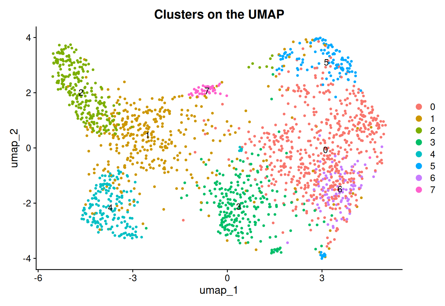
DimPlot(obj, group.by = "seurat_clusters", label = TRUE) + ggtitle("Clusters on the UMAP")

Eight clusters — but notice the shape. Unlike the well-separated islands of a mixed-tissue dataset, these clusters run together into one connected, branching manifold. That is exactly what a differentiating population looks like: each state melts into the next, and the branches are the beginnings of the committed fates. A continuous, branching UMAP like this is the visual signal that trajectory analysis is the right tool.

Fit the trajectory with Slingshot

Slingshot turns those clusters into lineages in two conceptual steps (Street et al., 2018):

1. Topology — an MST on the cluster centroids. It computes each cluster’s centre in the embedding and connects the centres with a minimum spanning tree: the shortest set of edges that links every cluster without a loop. That tree is the branching skeleton — which state flows into which.
2. Ordering — smooth principal curves. A tree of straight centroid-to-centroid segments is jagged, so Slingshot fits simultaneous principal curves through the actual cells along each root-to-tip path. Each curve is a smooth lineage, and a cell’s position along its curve is its pseudotime.

The call takes the embedding and the cluster labels. It also takes a root: Slingshot orders cells along the tree but cannot tell which end is the beginning, so left alone it infers a root — often landing on an undifferentiated cluster, but not guaranteed to be the one you mean. We know better here: the FACS labels tell us which cluster is the LT-HSC stem population, so we root the trajectory there with start.clus.

set.seed(42)
library(Seurat)
library(slingshot)
d <- readRDS("_data/nestorowa_hsc.rds")
obj <- CreateSeuratObject(counts = d$counts, meta.data = d$meta)
obj <- NormalizeData(obj, verbose = FALSE) |>
  FindVariableFeatures(nfeatures = 2000, verbose = FALSE) |> ScaleData(verbose = FALSE) |>
  RunPCA(npcs = 30, verbose = FALSE) |> RunUMAP(dims = 1:30, verbose = FALSE) |>
  FindNeighbors(dims = 1:30, verbose = FALSE) |> FindClusters(resolution = 0.6, verbose = FALSE)

# Which cluster is the stem-cell root? The one most enriched for LT-HSC in the FACS labels.
lthsc_frac <- prop.table(table(obj$seurat_clusters, obj$broad), 1)[, "LTHSC"]
root <- names(which.max(lthsc_frac))
round(sort(lthsc_frac, decreasing = TRUE), 3)   # LT-HSC fraction per cluster

    5     0     6     7     3     2     1     4 
0.578 0.343 0.192 0.075 0.070 0.070 0.052 0.035 

# Fit lineages + pseudotime on the UMAP, rooted at the LT-HSC cluster
sds <- slingshot(Embeddings(obj, "umap"),
                 clusterLabels = as.character(obj$seurat_clusters),
                 start.clus = root)

slingLineages(sds)               # the branching lineages, each a path of clusters from the root

$Lineage1
[1] "5" "0" "3" "1" "4"

$Lineage2
[1] "5" "0" "3" "1" "2"

$Lineage3
[1] "5" "0" "3" "1" "7"

$Lineage4
[1] "5" "0" "6"

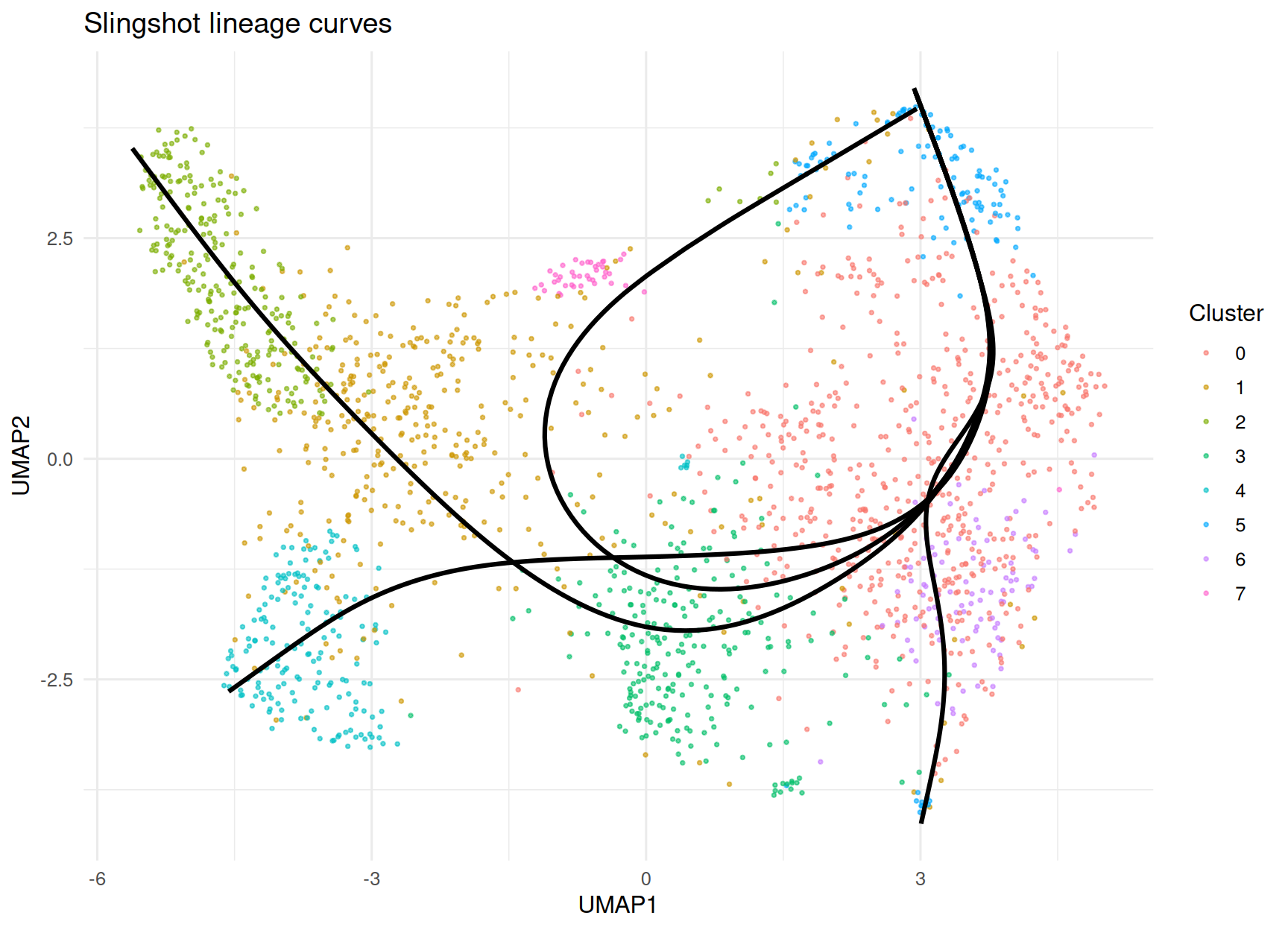
The most LT-HSC–enriched cluster (cluster 5, ~58% LT-HSC by FACS) is the root, and Slingshot resolves four lineages, all starting from it and fanning out to different tips — a stem population branching into several fates, exactly the tree hematopoiesis should produce. Each lineage is a path of clusters: they share an early trunk (5 → 0 → 3 → 1) and then split to distinct endpoints, plus one short branch (5 → 0 → 6) into an LMPP-enriched, lymphoid-primed cluster.

See the trajectory: lineage curves on the UMAP

The signature figure is the fitted lineage curves drawn over the cells. Pull the smooth curves out of the Slingshot object with slingCurves() and lay them on the UMAP: you see the branching skeleton the algorithm found, curving out of the root and splitting toward the fates.

set.seed(42)
library(Seurat)
library(slingshot)
library(ggplot2)
d <- readRDS("_data/nestorowa_hsc.rds")
obj <- CreateSeuratObject(counts = d$counts, meta.data = d$meta)
obj <- NormalizeData(obj, verbose = FALSE) |>
  FindVariableFeatures(nfeatures = 2000, verbose = FALSE) |> ScaleData(verbose = FALSE) |>
  RunPCA(npcs = 30, verbose = FALSE) |> RunUMAP(dims = 1:30, verbose = FALSE) |>
  FindNeighbors(dims = 1:30, verbose = FALSE) |> FindClusters(resolution = 0.6, verbose = FALSE)
root <- names(which.max(prop.table(table(obj$seurat_clusters, obj$broad), 1)[, "LTHSC"]))
sds  <- slingshot(Embeddings(obj, "umap"), clusterLabels = as.character(obj$seurat_clusters),
                  start.clus = root)

um <- Embeddings(obj, "umap")
cells <- data.frame(UMAP1 = um[, 1], UMAP2 = um[, 2], cluster = obj$seurat_clusters)
# Each fitted curve is a set of ordered points; pull them out for plotting
curves <- do.call(rbind, lapply(seq_along(slingCurves(sds)), function(i) {
  s <- slingCurves(sds)[[i]]$s[slingCurves(sds)[[i]]$ord, ]
  data.frame(UMAP1 = s[, 1], UMAP2 = s[, 2], lineage = paste0("Lineage ", i))
}))

ggplot(cells, aes(UMAP1, UMAP2)) +
  geom_point(aes(color = cluster), size = 0.6, alpha = 0.6) +
  geom_path(data = curves, aes(group = lineage), linewidth = 1.1) +
  labs(title = "Slingshot lineage curves", color = "Cluster") +
  theme_minimal(base_size = 12)

The four curves emerge from a single point — the LT-HSC root — and branch outward, each threading through the cells toward a different corner of the map. This is the whole idea of trajectory inference in one picture: a continuous, branching path fitted through a differentiating population, replacing hard cluster boundaries with the developmental structure that actually generated the cells.

Colour the map by pseudotime

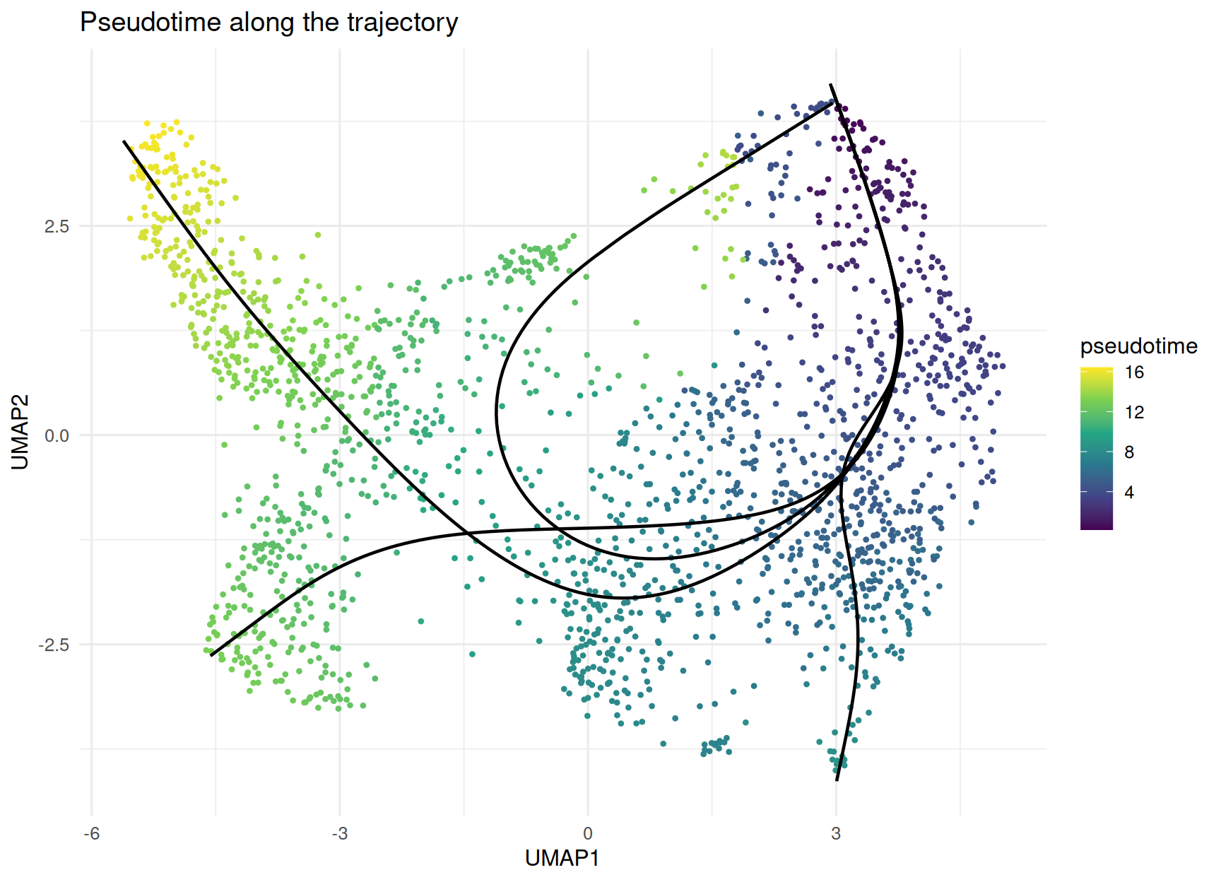
Each cell’s distance along its curve is its pseudotime. Averaging a cell’s pseudotime across the lineages it belongs to and colouring the UMAP by it shows the differentiation gradient directly: dark at the root, bright at the committed tips.

set.seed(42)
library(Seurat)
library(slingshot)
library(ggplot2)
d <- readRDS("_data/nestorowa_hsc.rds")
obj <- CreateSeuratObject(counts = d$counts, meta.data = d$meta)
obj <- NormalizeData(obj, verbose = FALSE) |>
  FindVariableFeatures(nfeatures = 2000, verbose = FALSE) |> ScaleData(verbose = FALSE) |>
  RunPCA(npcs = 30, verbose = FALSE) |> RunUMAP(dims = 1:30, verbose = FALSE) |>
  FindNeighbors(dims = 1:30, verbose = FALSE) |> FindClusters(resolution = 0.6, verbose = FALSE)
root <- names(which.max(prop.table(table(obj$seurat_clusters, obj$broad), 1)[, "LTHSC"]))
sds  <- slingshot(Embeddings(obj, "umap"), clusterLabels = as.character(obj$seurat_clusters),
                  start.clus = root)

pt <- slingPseudotime(sds)                    # cells x lineages
um <- Embeddings(obj, "umap")
cells <- data.frame(UMAP1 = um[, 1], UMAP2 = um[, 2],
                    pseudotime = rowMeans(pt, na.rm = TRUE))
curves <- do.call(rbind, lapply(seq_along(slingCurves(sds)), function(i) {
  s <- slingCurves(sds)[[i]]$s[slingCurves(sds)[[i]]$ord, ]
  data.frame(UMAP1 = s[, 1], UMAP2 = s[, 2], lineage = paste0("Lineage ", i))
}))

range(pt, na.rm = TRUE)                        # the pseudotime scale

[1]  0.00000 16.40755

ggplot(cells, aes(UMAP1, UMAP2, color = pseudotime)) +
  geom_point(size = 0.8) +
  geom_path(data = curves, aes(group = lineage), color = "black", linewidth = 0.8) +
  scale_color_viridis_c(na.value = "grey85") +
  labs(title = "Pseudotime along the trajectory") +
  theme_minimal(base_size = 12)

The pseudotime runs from 0 at the root to about 16 at the tips, and the gradient is smooth: no jump, just a steady progression outward along every branch. That continuity is the model — cells are ordered by how far they have differentiated, not sorted into stages.

Validate the trajectory against the known labels

A trajectory that looks plausible is not enough; check it against the biology you held back. Cross-tabulate the clusters against the FACS broad labels: the root cluster should be the stem-cell population, and the tip clusters should be the committed progenitors.

set.seed(42)
library(Seurat)
library(slingshot)
d <- readRDS("_data/nestorowa_hsc.rds")
obj <- CreateSeuratObject(counts = d$counts, meta.data = d$meta)
obj <- NormalizeData(obj, verbose = FALSE) |>
  FindVariableFeatures(nfeatures = 2000, verbose = FALSE) |> ScaleData(verbose = FALSE) |>
  RunPCA(npcs = 30, verbose = FALSE) |> RunUMAP(dims = 1:30, verbose = FALSE) |>
  FindNeighbors(dims = 1:30, verbose = FALSE) |> FindClusters(resolution = 0.6, verbose = FALSE)

# Cluster vs sorted population: does the root match LT-HSC and the tips match committed progenitors?
table(cluster = obj$seurat_clusters, FACS = obj$broad)

       FACS
cluster CMP GMP LMPP LTHSC MEP MPP
      0  39   9   94   191  15 209
      1 141  31   31    20 101  58
      2  19   3    0    18 216   2
      3  19   2  133    17   6  65
      4  76  71    2     6   3  12
      5   9   4   11    63   8  14
      6   3   1    9     5   3   5
      7  22   2    0     3  10   3

The story holds up. The root cluster (5) is dominated by LTHSC cells — the true apex stem cell — while the tips are committed progenitors: the erythroid/megakaryocyte endpoint (cluster 2) is ~84% MEP, the myeloid endpoint (cluster 4) is the most GMP-enriched, and the lymphoid trunk (cluster 3) is ~55% LMPP. Slingshot placed the stem cells at the start and the committed cells at the ends without ever seeing the FACS labels — the ordering it recovered from expression alone matches the known differentiation hierarchy. That agreement is your evidence the trajectory is real, not an artifact of the embedding.

Find genes that change along the trajectory with tradeSeq

The pseudotime is a means, not the end. The biological payoff is which genes drive the differentiation — the genes that switch on or off as cells travel each lineage. tradeSeq answers this: for each gene it fits a smooth generalized additive model (GAM) of expression against pseudotime, per lineage, then tests whether the gene varies significantly along the trajectory (Van den Berge et al., 2020).

fitGAM() does the fitting and associationTest() does the test. Fitting a GAM per gene is not free, so — as the tradeSeq authors recommend for a first pass — we fit the top 150 highly variable genes with 5 knots (the smoothness of the fitted curve); a real analysis scales this up. The pseudotime and per-cell lineage weights both come straight from the Slingshot object.

set.seed(42)
library(Seurat)
library(slingshot)
library(tradeSeq)
d <- readRDS("_data/nestorowa_hsc.rds")
sym <- d$symbol
obj <- CreateSeuratObject(counts = d$counts, meta.data = d$meta)
obj <- NormalizeData(obj, verbose = FALSE) |>
  FindVariableFeatures(nfeatures = 2000, verbose = FALSE) |> ScaleData(verbose = FALSE) |>
  RunPCA(npcs = 30, verbose = FALSE) |> RunUMAP(dims = 1:30, verbose = FALSE) |>
  FindNeighbors(dims = 1:30, verbose = FALSE) |> FindClusters(resolution = 0.6, verbose = FALSE)
root <- names(which.max(prop.table(table(obj$seurat_clusters, obj$broad), 1)[, "LTHSC"]))
sds  <- slingshot(Embeddings(obj, "umap"), clusterLabels = as.character(obj$seurat_clusters),
                  start.clus = root)

pt    <- slingPseudotime(sds, na = FALSE)      # cells x lineages, no NAs
cw    <- slingCurveWeights(sds)                # each cell's weight on each lineage
genes <- head(VariableFeatures(obj), 150)      # a fast first pass on the top 150 HVGs
set.seed(42)                                   # fitGAM initialization uses randomness — seed for a stable result
gam   <- fitGAM(counts = as.matrix(GetAssayData(obj, layer = "counts")[genes, ]),
                pseudotime = pt, cellWeights = cw, nknots = 5, verbose = FALSE)

assoc <- associationTest(gam)                  # test each gene for change along the lineages
assoc$symbol <- sym[rownames(assoc)]           # readable names
assoc <- assoc[order(assoc$pvalue), ]

sum(p.adjust(assoc$pvalue, "fdr") < 0.05, na.rm = TRUE)   # dynamic genes at 5% FDR

[1] 33

head(assoc[!is.na(assoc$symbol), c("symbol", "waldStat")], 10)

                    symbol waldStat
ENSMUSG00000051504 Siglech 127.2230
ENSMUSG00000105906   Iglc1 514.0457
ENSMUSG00000029373     Pf4 328.7270
ENSMUSG00000060586  H2-Eb1 206.4824
ENSMUSG00000036782  Klhl13 188.3286
ENSMUSG00000046826 Fam187b 123.0724
ENSMUSG00000061353  Cxcl12 196.5018
ENSMUSG00000038179  Slamf7 151.0669
ENSMUSG00000046818  Ddit4l 191.9911
ENSMUSG00000027524    Edn3 133.5374

Of the 150 genes tested, 33 vary significantly along the trajectory at a 5% false-discovery rate — genes whose expression is coupled to differentiation rather than flat. The top of the list is dominated by lineage-commitment and immune genes: the immunoglobulin gene Iglc1 (marking B-lymphoid commitment), the platelet factor Pf4 (a megakaryocyte-commitment gene), and the antigen-presentation gene H2-Eb1 (MHC class II). These are exactly the programs you expect to switch on as multipotent cells commit to specific blood fates.

Plot the dynamic genes along pseudotime

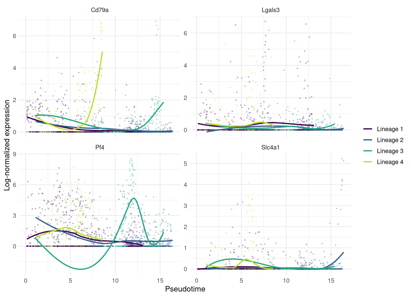
The clearest way to see a dynamic gene is to plot its expression against pseudotime, coloured by lineage. Pick one marker per fate — an erythroid gene, a megakaryocyte gene, a myeloid gene, a B-lymphoid gene — and each should light up in its own lineage and stay quiet in the others, the signature of fate-specific commitment.

set.seed(42)
library(Seurat)
library(slingshot)
library(ggplot2)
d <- readRDS("_data/nestorowa_hsc.rds")
sym <- d$symbol
obj <- CreateSeuratObject(counts = d$counts, meta.data = d$meta)
obj <- NormalizeData(obj, verbose = FALSE) |>
  FindVariableFeatures(nfeatures = 2000, verbose = FALSE) |> ScaleData(verbose = FALSE) |>
  RunPCA(npcs = 30, verbose = FALSE) |> RunUMAP(dims = 1:30, verbose = FALSE) |>
  FindNeighbors(dims = 1:30, verbose = FALSE) |> FindClusters(resolution = 0.6, verbose = FALSE)
root <- names(which.max(prop.table(table(obj$seurat_clusters, obj$broad), 1)[, "LTHSC"]))
sds  <- slingshot(Embeddings(obj, "umap"), clusterLabels = as.character(obj$seurat_clusters),
                  start.clus = root)

# Assign each cell to its strongest lineage and take that lineage's pseudotime
cw  <- slingCurveWeights(sds); pt <- slingPseudotime(sds, na = FALSE)
lin <- apply(cw, 1, which.max)
cell_pt <- pt[cbind(seq_len(nrow(pt)), lin)]

# One recognizable marker per fate (Ensembl IDs from the symbol map)
markers <- c(Slc4a1 = "ENSMUSG00000006574",  # erythroid
             Pf4    = "ENSMUSG00000029373",  # megakaryocyte
             Lgals3 = "ENSMUSG00000050335",  # myeloid
             Cd79a  = "ENSMUSG00000003379")  # B-lymphoid
logn <- GetAssayData(obj, layer = "data")
plotdf <- do.call(rbind, lapply(names(markers), function(g)
  data.frame(pseudotime = cell_pt, lineage = paste0("Lineage ", lin),
             expression = as.numeric(logn[markers[g], ]), gene = g)))

ggplot(plotdf, aes(pseudotime, expression, color = lineage)) +
  geom_point(size = 0.4, alpha = 0.25) +
  geom_smooth(se = FALSE, method = "loess", formula = y ~ x, linewidth = 0.9) +
  facet_wrap(~ gene, scales = "free_y") +
  scale_color_viridis_d(end = 0.9) +
  labs(x = "Pseudotime", y = "Log-normalized expression", color = NULL) +
  theme_minimal(base_size = 12)

Each marker turns on in a different lineage, and the cleanest cases track the progenitor identity at the branch tip: the erythroid gene Slc4a1 climbs late in the lineage that ends in the MEP-dominated cluster, and the myeloid gene Lgals3 rises in the lineage that ends in the GMP-enriched cluster. The megakaryocyte gene Pf4 and the B-lymphoid gene Cd79a each peak in a different branch again — a reminder that not every inferred tip is a textbook committed fate: two of these lineages end in mixed progenitor clusters (a CMP-plurality and an LMPP-primed cluster), so the markers report lineage bias, not a clean terminal cell type. That is both the power and the honest limit of trajectory analysis: it reveals not just that cells differentiate, but which genes rise along each branch and when — as sharply as your clustering resolves the branches (see the caveats below).

Honest caveats: what pseudotime is and is not

Trajectory inference is powerful and easy to over-read. Keep four things straight:

• Pseudotime is not real time. It orders cells by transcriptional progression, not by clock hours. Two cells at pseudotime 5 and 10 differ in maturity, but nothing says the second took twice as long. Never quote pseudotime as a duration.
• It needs a genuine continuum. Slingshot will happily fit a tree to any set of clusters, including discrete, unrelated cell types — and hand you a meaningless ordering. The method cannot tell you whether a trajectory exists; that is your call, made before you run it. If your UMAP is well-separated islands, not a connected manifold, there is no trajectory to infer.
• The root sets the direction, and choosing it wrong flips the story. Slingshot recovers the topology and the ordering along it, but not which end is the start. Left to infer the root it may pick the wrong cluster, reversing a lineage so genes look switched off during differentiation when they switch on. Anchor the root in real knowledge — here the FACS stem-cell label — whenever you have it (start.clus).
• Topology and ordering are not the same as directionality. Even correctly rooted, Slingshot infers direction from your choice of root, not from the data. Reading direction out of the data itself needs RNA velocity (from the ratio of unspliced to spliced transcripts) — a Python-first method (scVelo) with no first-class R equivalent, covered in a companion lesson on RNA velocity and fate mapping. A separate companion lesson covers Monocle3, a graph-based alternative that learns a principal graph for more complex or disconnected topologies. Slingshot is the clean, R-native default for the common branching case.

Which method when

You have…	Use	Why
A differentiating population with a clear branching structure, in R	Slingshot (+ tradeSeq)	MST + principal curves on your existing embedding; simple, robust, Seurat/SCE-native
A complex or disconnected topology (loops, many branches)	Monocle3 (companion lesson)	Learns a principal graph, not just a tree; its own graph_test for dynamic genes
A need to infer direction from the data, not a known root	RNA velocity (scVelo, Python; companion lesson)	Uses spliced/unspliced ratios to point the arrow of differentiation
Discrete, stable cell types (no continuum)	None — annotate instead	There is no developmental path to order along; use cell-type annotation

The through-line: Slingshot orders cells along a trajectory you have judged to be real; tradeSeq finds the genes that change along it; and the root — from biology — sets the direction.

Common issues

The lineages point the wrong way, or the root is on a mature cluster. Slingshot inferred the root and guessed wrong. It orders cells along the tree but does not know biology — so tell it: pass start.clus = the cluster you know is the origin (here the LT-HSC–enriched cluster, identified from the FACS labels). With the right root, every lineage runs from stem to committed, and the gene dynamics read in the correct direction.

Too many or too few lineages. The number of branches is driven by the clustering, because the MST is built on cluster centroids. Over-clustering (a high FindClusters resolution) fragments one fate into several tips and invents spurious branches; under-clustering merges real fates. If the lineage count does not match the known biology, adjust the clustering resolution before blaming Slingshot — the trajectory is only as good as the clusters underneath it.

Pseudotime is NA for some cells. A cell that belongs to one lineage has no pseudotime on the others, so slingPseudotime() returns NA there by design. For a per-cell value (e.g. to colour a plot), either average across lineages with rowMeans(pt, na.rm = TRUE), or assign each cell to its strongest lineage with slingCurveWeights() and take that lineage’s pseudotime. Pass na = FALSE to slingPseudotime() when a downstream tool (like tradeSeq) needs a complete matrix.

Frequently asked questions

NoteWhat is pseudotime in single-cell RNA-seq?

Pseudotime is a number assigned to each cell that measures how far it has progressed along a developmental trajectory, inferred from how gradually its gene expression changes relative to other cells. Cells at the start of differentiation get low values and fully committed cells get high ones. It is not measured in real time (hence pseudo); it captures ordering and maturity, not duration. Use it when your cells form a genuine continuum, such as stem cells differentiating into mature types.

NoteHow does Slingshot infer a trajectory?

Slingshot works in two steps. First it builds a minimum spanning tree on the cluster centroids in your low-dimensional embedding to find the branching topology — which cell state connects to which. Then it fits smooth principal curves through the cells along each root-to-tip path, and a cell’s position along its curve is its pseudotime. You call it with slingshot(embedding, clusterLabels = clusters, start.clus = root), giving it an embedding (like UMAP or PCA), your cluster labels, and the starting cluster.

NoteSlingshot vs Monocle3 — which should I use?

Slingshot fits a minimum spanning tree on clusters and smooth curves — simple, robust, R/Seurat-native, and ideal for a clear branching differentiation. Monocle3 learns a principal graph and handles more complex or disconnected topologies (loops, many branches) with its own graph_test for dynamic genes. For a straightforward tree-shaped trajectory, Slingshot is the clean default; reach for Monocle3 when the topology is genuinely complex. A companion lesson covers Monocle3 in depth.

NoteHow do I find genes that change along a trajectory?

Use tradeSeq after Slingshot. It fits a smooth generalized additive model (GAM) of each gene’s expression against pseudotime per lineage with fitGAM(), then associationTest() tests which genes vary significantly along the trajectory. Feed it the pseudotime (slingPseudotime(sds, na = FALSE)) and per-cell lineage weights (slingCurveWeights(sds)) from the Slingshot object. The significant genes are the ones whose expression is coupled to differentiation.

NoteDoes Slingshot tell me the direction of differentiation?

No — Slingshot recovers the topology (the branching tree) and the ordering along it, but it cannot tell which end is the beginning. You supply the direction by setting the root cluster (start.clus) from biological knowledge, such as a known stem-cell marker or a FACS label. Inferring direction from the data itself requires RNA velocity (scVelo), which uses the ratio of unspliced to spliced transcripts and is a Python-first method covered in a companion lesson.

Test your understanding

ImportantYour turn: re-root the trajectory and watch it flip

Using nestorowa_hsc.rds, build the clusters and run Slingshot twice: once rooted at the LT-HSC–enriched cluster (as in the lesson), and once rooted at the most MEP-enriched cluster (a committed tip). Compare slingLineages() and the pseudotime of a few LT-HSC cells between the two. What happens to the ordering, and why is the root choice not a cosmetic detail?

TipHint

The only change is start.clus. Find the MEP-enriched cluster the same way you found the LT-HSC one: names(which.max(prop.table(table(obj$seurat_clusters, obj$broad), 1)[, "MEP"])). Then compare slingPseudotime(sds_stem) against slingPseudotime(sds_mep) for the stem cells — a cell that was near pseudotime 0 in one rooting will be near the maximum in the other.

TipSolution

set.seed(42)
library(Seurat); library(slingshot)
d <- readRDS("_data/nestorowa_hsc.rds")
obj <- CreateSeuratObject(counts = d$counts, meta.data = d$meta)
obj <- NormalizeData(obj, verbose = FALSE) |>
  FindVariableFeatures(nfeatures = 2000, verbose = FALSE) |> ScaleData(verbose = FALSE) |>
  RunPCA(npcs = 30, verbose = FALSE) |> RunUMAP(dims = 1:30, verbose = FALSE) |>
  FindNeighbors(dims = 1:30, verbose = FALSE) |> FindClusters(resolution = 0.6, verbose = FALSE)
emb <- Embeddings(obj, "umap"); cl <- as.character(obj$seurat_clusters)
fac <- prop.table(table(obj$seurat_clusters, obj$broad), 1)

stem_root <- names(which.max(fac[, "LTHSC"]))
mep_root  <- names(which.max(fac[, "MEP"]))
sds_stem  <- slingshot(emb, clusterLabels = cl, start.clus = stem_root)
sds_mep   <- slingshot(emb, clusterLabels = cl, start.clus = mep_root)

slingLineages(sds_stem)     # lineages run stem -> committed
slingLineages(sds_mep)      # lineages now run committed -> ... (reversed / re-rooted)

Re-rooting reverses the reading of the trajectory: the cells Slingshot placed at pseudotime 0 with the stem root sit at the far end with the MEP root. The curves are similar, but the direction — and therefore whether a gene reads as switching on or off during differentiation — depends entirely on the root. That is why you anchor the root in real biology, not on Slingshot’s default guess.

NoteQuick check: your UMAP shows three well-separated, non-touching islands of cells (monocytes, T cells, B cells). You run Slingshot and get a pseudotime. Is it meaningful?

A. Yes — Slingshot ran without error, so the ordering is valid. B. No — these are discrete, stable cell types with no developmental continuum between them, so there is no trajectory to order along; Slingshot fits a tree regardless, but the pseudotime is meaningless. C. Yes, but only if you set the root correctly.

TipShow answer

B. Slingshot will always fit a minimum spanning tree and return a pseudotime — it cannot tell you whether a trajectory exists. Monocytes, T cells and B cells are separate mature lineages, not points on one differentiation path, so ordering them along a pseudotime is meaningless no matter how you root it. Trajectory analysis is for genuine continua; deciding you have one is a judgement you make before running the method, by looking for a connected, branching manifold rather than separate islands.

Conclusion

Some biology is a gradient, and clustering flattens it. Trajectory analysis recovers the gradient: Slingshot builds a minimum spanning tree on your clusters and smooths it into branching lineage curves, and the position of each cell along its curve is its pseudotime. On the Nestorowa blood dataset it resolved four lineages fanning out of a single stem-cell root — and cross-checking against the held-back FACS labels confirmed the root really is the LT-HSC population and the tips really are committed progenitors. Then tradeSeq found the 33 genes that change along the trajectory, and plotting fate markers against pseudotime showed each blood program — erythroid, megakaryocyte, myeloid, lymphoid — switching on in its own lineage. The discipline is what matters: confirm you have a continuum before you start, root the trajectory in real biology so the direction is right, and remember that pseudotime is an ordering, not a clock — and that reading direction from the data itself is the job of RNA velocity, not Slingshot.

Related lessons

• Clustering & UMAP — builds the clusters and the embedding Slingshot fits the trajectory on; a good trajectory starts with sensible clusters. · Marker genes & cell-type annotation — the discrete counterpart: label stable cell types, the question trajectory analysis explicitly does not answer. · Pseudobulk differential expression — the other “which genes change” analysis, but across conditions rather than along a trajectory. · Bioinformatics — the pillar.
• Where this fits: clustering & UMAP → marker genes & annotation → trajectory & pseudotime with Slingshot → genes-along-lineage with tradeSeq — from a static map of cell types to the dynamic path between them.

🟢 With an AI agent

Ask Prova “how do I run Slingshot pseudotime on my own Seurat object and set the root cluster, then find genes that change along the trajectory with tradeSeq?” — it answers with R code you can run on your own data: cluster and embed, call slingshot() with start.clus, read the lineages, and fit tradeSeq. The runtime is the judge. Ask Prova →

Was this page helpful?

Prove you can do it. Master the whole Single-Cell RNA-Seq Analysis in R series — track your path, build projects, and earn a certificate.

Start free →

Go Pro — unlimited Prova on your own data and a verifiable certificate that proves the skill.

from $15/mo billed yearly

Go Pro →

✓ You're Pro — keep going. The runtime is the judge.

Get new R & Python lessons by email

Practical, reproducible, no spam. Unsubscribe anytime.

Double opt-in. We never share your email.

Share this pageXLinkedInRedditHN

Note

This lesson is reproducible: every figure and number was produced by the code shown — copy any block and run it to reproduce them. The runtime is the judge.

References

• Street, K., et al. (2018). Slingshot: cell lineage and pseudotime inference for single-cell transcriptomics. BMC Genomics, 19, 477. https://doi.org/10.1186/s12864-018-4772-0
• Van den Berge, K., et al. (2020). Trajectory-based differential expression analysis for single-cell sequencing data (tradeSeq). Nature Communications, 11, 1201. https://doi.org/10.1038/s41467-020-14766-3
• Nestorowa, S., et al. (2016). A single-cell resolution map of mouse hematopoietic stem and progenitor cell differentiation — the source of the HSPC dataset. Blood, 128(8), e20–e31. https://doi.org/10.1182/blood-2016-05-716480
• Saelens, W., et al. (2019). A comparison of single-cell trajectory inference methods. Nature Biotechnology, 37, 547–554. https://doi.org/10.1038/s41587-019-0071-9