Slingshot vs Monocle3: Which Trajectory Method to Use in R

See both methods run on the same cells side by side, then use a clear decision framework to pick the right trajectory-inference tool for your data

A practical, side-by-side comparison of Slingshot and Monocle3 for single-cell trajectory inference in R. Fit both on the same Nestorowa blood stem-cell dataset, see how a minimum spanning tree of principal curves differs from a learned principal graph — one connected tree versus separate partitions — and get a decision framework for choosing a pseudotime method, plus where lightweight (TSCAN) and multi-condition (condiments) options fit.

TipKey takeaways

• Same goal, two philosophies. Both order cells along a differentiation continuum and hand you a pseudotime, but Slingshot fits a minimum spanning tree (MST) on cluster centroids and smooths it into principal curves (Street et al., 2018), while Monocle3 learns a principal graph through the cells with reversed graph embedding (Cao et al., 2019).
• The sharpest practical difference is how they treat disconnected cells. Slingshot forces every cell onto one connected tree — everyone gets a pseudotime. Monocle3 splits cells into partitions and gives cells on a disconnected component infinite pseudotime, refusing to invent a path the data does not show.
• They also disagree on the embedding. Slingshot runs on your existing embedding (the Seurat UMAP); Monocle3 builds and runs on its own UMAP inside a cell_data_set. So the two trajectories are fitted on slightly different maps of the same cells.
• Pick by topology and honesty needs, not by fashion. Use Slingshot for a clean branching tree on an embedding you already trust; reach for Monocle3 when the topology is complex or you want the method to flag cells that are not on the trajectory.
• On a hard dataset, run both. Where they agree, trust the trajectory; where they disagree — usually about whether cells form one continuum or several — the disagreement is itself the finding.

Introduction

You have now met both single-cell trajectory-inference methods in depth: the Slingshot lesson fitted branching lineage curves and found dynamic genes with tradeSeq, and the Monocle3 lesson learned a principal graph and tested genes with Moran’s I. Each works. The question this lesson answers is the one you actually face at the bench: given a dataset, which do you reach for?

The honest way to decide is to run both on the same cells and look at where they agree and where they part. So that is what we do. On one differentiating blood dataset we fit a Slingshot trajectory and a Monocle3 trajectory, put them side by side, and read off the structural contrast directly from the figure — not from a table of claims. Then we turn that contrast into a decision framework: a comparison table and a plain “use Slingshot when… / use Monocle3 when…” rule you can apply to your own data. We close with two options the two headline methods leave on the table — a lightweight single-cell-experiment-native baseline (TSCAN) and a tool for comparing trajectories across conditions (condiments).

This is a static comparison lesson: the two deep-dive lessons carry the full, step-by-step walkthroughs (rooting, validation against known labels, gene testing). Here we fit just enough of each to see the difference and choose. If you want the complete pipeline for either method, follow its own lesson.

We use the same data as both deep dives so the comparison is apples to apples: the canonical Nestorowa mouse blood dataset (Nestorowa et al., 2016) — 1,920 hematopoietic stem and progenitor cells (HSPCs — the stem and progenitor cells that produce every blood cell), each carrying a FACS label (fluorescence-activated cell sorting — the flow-cytometry gating that sorted the cells by surface markers) recording which progenitor population it belongs to.

Fit Slingshot on the cells

First, the Slingshot side, exactly as in its own lesson but stopping at the pseudotime — no gene testing here. We run the standard single-cell RNA-seq (scRNA-seq) pipeline in Seurat — normalize, find variable genes, reduce with principal component analysis (PCA), build a UMAP (uniform manifold approximation and projection, the 2-D map), and cluster — then call slingshot() on the Seurat UMAP with the cluster labels, rooted at the long-term stem-cell cluster we read from the FACS labels. A fixed seed keeps the clustering and embedding reproducible.

set.seed(42)
library(Seurat)
library(slingshot)
library(ggplot2)

d <- readRDS("_data/nestorowa_hsc.rds")
obj <- CreateSeuratObject(counts = d$counts, meta.data = d$meta)
obj <- NormalizeData(obj, verbose = FALSE) |>
  FindVariableFeatures(nfeatures = 2000, verbose = FALSE) |> ScaleData(verbose = FALSE) |>
  RunPCA(npcs = 30, verbose = FALSE) |> RunUMAP(dims = 1:30, verbose = FALSE) |>
  FindNeighbors(dims = 1:30, verbose = FALSE) |> FindClusters(resolution = 0.6, verbose = FALSE)

# Root at the most LT-HSC-enriched cluster (LT-HSC = long-term hematopoietic stem cell, the apex stem cell)
root <- names(which.max(prop.table(table(obj$seurat_clusters, obj$broad), 1)[, "LTHSC"]))
sds  <- slingshot(Embeddings(obj, "umap"),
                  clusterLabels = as.character(obj$seurat_clusters),
                  start.clus = root)

length(slingLineages(sds))          # how many lineages Slingshot resolved

[1] 4

sum(!is.nan(rowMeans(slingPseudotime(sds), na.rm = TRUE)))   # how many cells got a pseudotime

[1] 1920

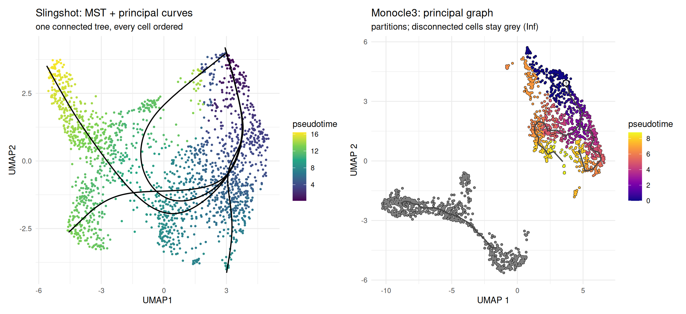
Slingshot resolves a handful of lineages, all fanning out from the single stem-cell root, and — the point to hold onto — every cell receives a pseudotime. Slingshot builds one connected tree and orders all 1,920 cells along it; nothing is left off. We build the plot object now and draw it side by side with Monocle3 in a moment.

# Package the Slingshot result as a ggplot: cells coloured by pseudotime + the lineage curves
um <- Embeddings(obj, "umap")
pt_sling <- rowMeans(slingPseudotime(sds), na.rm = TRUE)
cells <- data.frame(UMAP1 = um[, 1], UMAP2 = um[, 2], pseudotime = pt_sling)
curves <- do.call(rbind, lapply(seq_along(slingCurves(sds)), function(i) {
  s <- slingCurves(sds)[[i]]$s[slingCurves(sds)[[i]]$ord, ]
  data.frame(UMAP1 = s[, 1], UMAP2 = s[, 2], lineage = paste0("L", i))
}))

p_sling <- ggplot(cells, aes(UMAP1, UMAP2, color = pseudotime)) +
  geom_point(size = 0.7) +
  geom_path(data = curves, aes(group = lineage), color = "black", linewidth = 0.7) +
  scale_color_viridis_c(na.value = "grey85") +
  labs(title = "Slingshot: MST + principal curves", subtitle = "one connected tree, every cell ordered") +
  theme_minimal(base_size = 11)

Fit Monocle3 on the same cells

Now the Monocle3 side, from its own lesson. Monocle3 does not take a Seurat object; it works on a cell_data_set (a CDS — its container built on Bioconductor’s SingleCellExperiment, SCE). And it does not reuse the Seurat UMAP — it runs its own preprocess_cds() → reduce_dimension() → cluster_cells() pipeline, then learn_graph() fits the principal graph and order_cells() roots it at the stem cells. We root it programmatically (never the interactive picker) so the render is reproducible.

# learn_graph() prints a progress bar; run the whole Monocle3 fit quietly and read the result below.
set.seed(42)
library(monocle3)

d <- readRDS("_data/nestorowa_hsc.rds")
gene_meta <- data.frame(gene_short_name = d$symbol[rownames(d$counts)],
                        row.names = rownames(d$counts))
cds <- new_cell_data_set(d$counts, cell_metadata = d$meta, gene_metadata = gene_meta)

set.seed(42); cds <- preprocess_cds(cds, num_dim = 30)              # PCA
set.seed(42); cds <- reduce_dimension(cds, reduction_method = "UMAP")
set.seed(42); cds <- cluster_cells(cds)
cds <- learn_graph(cds)

# Root programmatically at the LT-HSC stem cells (the documented get_earliest_root pattern)
get_earliest_root <- function(cds, cell_col, target) {
  cell_ids <- which(colData(cds)[[cell_col]] == target)
  closest <- principal_graph_aux(cds)[["UMAP"]]$pr_graph_cell_proj_closest_vertex
  igraph::V(principal_graph(cds)[["UMAP"]])$name[
    as.numeric(names(which.max(table(closest[cell_ids, ]))))]
}
cds <- order_cells(cds, root_pr_nodes = get_earliest_root(cds, "broad", "LTHSC"))

length(unique(partitions(cds)))     # how many separate manifolds Monocle3 found

[1] 2

sum(is.finite(pseudotime(cds)))     # how many cells got a FINITE pseudotime

[1] 1138

Read those two numbers against Slingshot’s. Monocle3 splits the cells into more than one partition — groups it judges to sit on separate manifolds — and only the cells reachable from the root get a finite pseudotime. A large block of cells is left at infinite pseudotime: Monocle3 is telling you it does not see those cells as part of this trajectory. That is the structural fork between the two methods, and the next figure makes it visible.

# plot_cells() returns a ggplot: the principal graph over Monocle3's own UMAP, coloured by pseudotime
p_mono <- plot_cells(cds, color_cells_by = "pseudotime",
                     label_cell_groups = FALSE, label_leaves = FALSE,
                     label_branch_points = FALSE, cell_size = 0.7) +
  labs(title = "Monocle3: principal graph", subtitle = "partitions; disconnected cells stay grey (Inf)") +
  theme_minimal(base_size = 11)

The side-by-side: one connected tree vs separate partitions

Here is the whole comparison in one figure — the same 1,920 cells, Slingshot on the left and Monocle3 on the right, each coloured by its own pseudotime. Do not compare the two colour scales directly (pseudotime has no units and each method sets its own range); compare the structure.

library(patchwork)
p_sling + p_mono

The contrast is immediate. Slingshot (left) covers every cell in colour: it committed to one connected tree and gave all 1,920 cells a place on it. Monocle3 (right) roots and colours the main body of cells but leaves a whole block grey — the disconnected partition it refused to order. Same cells, same biology, two different answers to the same question: is this one continuum or several? Slingshot answers “one, always”; Monocle3 answers “as many as the data supports, and here it is more than one.”

Neither answer is automatically right. Slingshot’s is convenient and often correct when you already know the cells form a single differentiating population. Monocle3’s is more cautious and more honest when you are not sure — it surfaces the question instead of silently deciding for you. Which behaviour you want is the core of the choice, and it is what the decision framework below turns into a rule.

The decision framework

The two methods differ on six axes that actually matter in practice. This table is the reference to keep:

	Slingshot	Monocle3
What it fits	An MST on cluster centroids, smoothed into principal curves	A principal graph learned through the cells with reversed graph embedding (RGE)
Embedding	Your existing embedding (the Seurat/SCE UMAP) + your cluster labels	Its own UMAP, built inside the cell_data_set
Topology	A tree — branches from a root, no loops	A graph — can branch, converge, or loop
Disconnected cells	Forced into the tree; every cell gets a pseudotime	Split into partitions; off-graph cells get infinite pseudotime
Dynamic-gene test	tradeSeq — a generalized additive model (GAM) of expression vs pseudotime, per lineage	graph_test() — Moran’s I spatial autocorrelation over the graph
Object & ecosystem	Runs on a matrix + labels; Seurat/SCE-native, one call slingshot()	A cell_data_set container; a pipeline of verbs with its own plotting

Read the table as a single story. Slingshot is lighter and more composable: it slots onto an embedding you already built and trust, it is one function call, and it never leaves a cell behind. Monocle3 is more expressive and more opinionated: it owns the whole pipeline from its own dimension reduction to its own graph and plots, it can express topologies a tree cannot, and it will tell you — via partitions and infinite pseudotime — when it thinks some cells do not belong.

Use Slingshot when…

• You already have a good embedding and clusters (from Seurat or a SingleCellExperiment) that you trust, and you want to fit the trajectory on that map rather than a new one.
• The biology is a clear branching tree — one origin fanning out to a few fates — with no loops and no suspicion of disconnected populations.
• You want a simple, robust, one-call method that stays inside the Seurat/SCE ecosystem, and you plan to test dynamic genes per lineage with tradeSeq.

Use Monocle3 when…

• The topology is complex — many branches, a convergence, or a possible loop — and a tree would oversimplify it.
• You suspect disconnected populations (a contaminating cell type, two separate manifolds) and you want the method to flag them rather than force them onto one path. Monocle3’s partitions are the feature.
• You want an all-in-one pipeline with its own embedding, graph, plotting, and a Moran’s-I dynamic-gene test (graph_test()), and you are comfortable working in the cell_data_set world.

And when a dataset is genuinely hard, run both. Where the two agree, the trajectory is robust to the method. Where they disagree — most often about whether the cells are one continuum or several — Monocle3’s partitions usually explain why, and the disagreement is a result worth reporting, not a nuisance to reconcile away.

Lightweight and multi-condition options

The two headline methods are not the only tools. Two more are worth knowing, and the code below is illustrative — neither package is installed in this lesson’s render image, so the snippets are marked eval: false. Run them in your own environment.

TSCAN — the lightweight, SCE-native baseline

If you want the simplest possible trajectory — an MST on cluster centroids, no more — TSCAN (Ji & Ji, 2016) is the minimal Bioconductor option. Its quickPseudotime() wraps the whole MST pipeline on a SingleCellExperiment, and testPseudotime() tests genes along a path with a spline model. It is conceptually close to Slingshot’s first step (the MST) without the principal-curve smoothing — a good baseline when you want something fast and transparent.

# Illustrative — TSCAN is NOT installed in this lesson's image.
# Install in your own environment: BiocManager::install("TSCAN")
library(TSCAN)

# `sce` is a SingleCellExperiment with a reduced dimension (e.g. "PCA") and a
# `clusters` vector. quickPseudotime() runs aggregateAcrossCells() -> MST -> orderCells():
out <- quickPseudotime(sce, clusters = clusters, use.dimred = "PCA")

out$mst                       # the minimum spanning tree on cluster centroids
head(out$ordering)            # per-cell pseudotime, one column per path

# Test which genes change along the first path with a spline model:
res <- testPseudotime(sce, pseudotime = out$ordering[, 1])

condiments — comparing trajectories across conditions

Slingshot, Monocle3, and TSCAN all fit one trajectory. When your experiment has multiple conditions (treated vs control, mutant vs wild-type) and you want to ask whether the trajectory itself differs between them — different topology, different progression, different differentiation, different expression — condiments (Roux de Bézieux et al., 2024) is the framework built for that. It sits on top of a fitted trajectory (typically Slingshot) and adds condition-level tests.

# Illustrative — condiments is NOT installed in this lesson's image.
# Install in your own environment: BiocManager::install("condiments")
library(condiments)

# `sds` is a Slingshot result; `condition` is a per-cell factor (e.g. treated / control).
# Does the trajectory topology itself differ between conditions?
topologyTest(sds, conditions = condition)

# Do cells progress along the trajectory at different rates between conditions?
progressionTest(sds, conditions = condition)

Reach for condiments only when comparing conditions is the actual question; for a single-sample trajectory, Slingshot or Monocle3 alone is the right scope.

Common issues

The two methods disagree on the number of trajectories — which is right? Neither, automatically. The count depends on choices upstream of the method: Slingshot’s branch count comes from your clustering resolution (the MST is built on cluster centroids), while Monocle3’s comes from its partitions and the learned graph. A disagreement usually means the two are answering slightly different questions about connectivity. Check the biology: cross-tabulate clusters against known labels (FACS, marker genes) and decide how many fates you actually expect, then judge each method against that rather than against each other.

The pseudotime values are on completely different scales. They are supposed to be. Pseudotime has no units and each method sets its own range — Slingshot’s might run 0–16 while Monocle3’s runs 0–9 on the same cells. Never compare the raw numbers across methods (or even across two runs of one method). Compare orderings and structure: which cells are early vs late, and which genes rise along the path. If you must put two pseudotimes on one axis, rank-transform or min–max scale each to [0, 1] first.

Which embedding should I trust — my Seurat UMAP or Monocle3’s own? Both are valid 2-D projections of the same PCA-reduced data; they differ because UMAP is stochastic and each tool runs it with different defaults and seeds. Slingshot fits on the embedding you give it (so you control it); Monocle3 fits on the one it builds. For a fair visual comparison, remember you are looking at two maps, not one — the cells are identical, but their 2-D coordinates are not. Trust the embedding whose global structure best matches your known biology, and report which one each trajectory was fitted on.

Frequently asked questions

NoteIs Slingshot or Monocle3 better for trajectory analysis?

Neither is universally better — they suit different situations. Slingshot is simpler, runs on your existing embedding, fits a minimum spanning tree smoothed into principal curves, and forces every cell onto one connected tree; it is ideal for a clear branching differentiation in R. Monocle3 learns a principal graph on its own UMAP, can express more complex topologies (loops, convergence), and uses partitions to keep disconnected cells off the trajectory rather than forcing them on. Choose Slingshot for a clean tree on an embedding you trust; choose Monocle3 for complex or possibly-disconnected topologies, or when you want the method to flag cells that are not on the trajectory.

NoteCan I use both Slingshot and Monocle3 on the same data?

Yes, and on a hard dataset it is good practice. Run both, then compare the orderings and the inferred topology. Where they agree, the trajectory is robust to the choice of method and you can trust it. Where they disagree — most commonly about whether the cells form one continuum or several — the disagreement is itself informative: Monocle3’s partitions often explain the gap. Just do not compare the raw pseudotime values across the two, since each sets its own arbitrary scale.

NoteWhich method should I use for a branching trajectory?

For a straightforward branching tree — one origin fanning out to a few committed fates, no loops — Slingshot is the clean default: it fits exactly that shape (an MST plus principal curves) with a single function call on your existing embedding. Reach for Monocle3 when the branching is more complex than a tree (converging paths, loops) or when you suspect some branches are actually disconnected populations, because its principal graph and partitions handle those cases where a tree cannot.

NoteWhy do Slingshot and Monocle3 give different pseudotime values?

Because they build the trajectory differently and set independent scales. Slingshot smooths principal curves on your UMAP and measures distance along each curve; Monocle3 learns a graph on its own UMAP and measures distance along the graph. The two use different embeddings, different skeletons, and different units, so the numbers will not match even when the ordering agrees. Compare the relative ordering of cells and the genes that change along the path, not the absolute pseudotime values.

NoteWhat is a lightweight alternative to Slingshot and Monocle3?

TSCAN (Ji & Ji, 2016) is the minimal option: it builds a minimum spanning tree on cluster centroids and orders cells along it, all wrapped in one quickPseudotime() call on a SingleCellExperiment, with testPseudotime() for genes along a path. It is conceptually Slingshot’s MST step without the principal-curve smoothing — fast and transparent, and a sensible baseline. For comparing trajectories across conditions, use condiments (Roux de Bézieux et al., 2024) on top of a fitted trajectory.

Test your understanding

ImportantYour turn: quantify the disagreement

Using nestorowa_hsc.rds, fit both trajectories on the same cells (the two pipelines from this lesson), then compute a single number for each method: how many of the 1,920 cells get a finite pseudotime? Compare the two counts. What does the gap between them tell you, and which method is being more cautious about the structure of the data?

TipHint

For Slingshot, a cell has a pseudotime if rowMeans(slingPseudotime(sds), na.rm = TRUE) is not NaN — but in practice Slingshot orders all cells, so the count is 1,920. For Monocle3, count with sum(is.finite(pseudotime(cds))) after order_cells() — cells in a disconnected partition are Inf. The gap between the two counts is exactly the set of cells Monocle3 held off the trajectory.

TipSolution

set.seed(42)
library(Seurat); library(slingshot); library(monocle3)
d <- readRDS("_data/nestorowa_hsc.rds")

# --- Slingshot: every cell is forced onto the tree ---
obj <- CreateSeuratObject(counts = d$counts, meta.data = d$meta)
obj <- NormalizeData(obj, verbose = FALSE) |>
  FindVariableFeatures(nfeatures = 2000, verbose = FALSE) |> ScaleData(verbose = FALSE) |>
  RunPCA(npcs = 30, verbose = FALSE) |> RunUMAP(dims = 1:30, verbose = FALSE) |>
  FindNeighbors(dims = 1:30, verbose = FALSE) |> FindClusters(resolution = 0.6, verbose = FALSE)
root <- names(which.max(prop.table(table(obj$seurat_clusters, obj$broad), 1)[, "LTHSC"]))
sds  <- slingshot(Embeddings(obj, "umap"), clusterLabels = as.character(obj$seurat_clusters),
                  start.clus = root)
sum(!is.nan(rowMeans(slingPseudotime(sds), na.rm = TRUE)))   # ~1920 — all cells ordered

# --- Monocle3: partitions leave the disconnected cells at Inf ---
gene_meta <- data.frame(gene_short_name = d$symbol[rownames(d$counts)], row.names = rownames(d$counts))
cds <- new_cell_data_set(d$counts, cell_metadata = d$meta, gene_metadata = gene_meta)
set.seed(42); cds <- preprocess_cds(cds, num_dim = 30)
set.seed(42); cds <- reduce_dimension(cds, reduction_method = "UMAP")
set.seed(42); cds <- cluster_cells(cds); cds <- learn_graph(cds)
get_earliest_root <- function(cds, cell_col, target) {
  ids <- which(colData(cds)[[cell_col]] == target)
  closest <- principal_graph_aux(cds)[["UMAP"]]$pr_graph_cell_proj_closest_vertex
  igraph::V(principal_graph(cds)[["UMAP"]])$name[as.numeric(names(which.max(table(closest[ids, ]))))]
}
cds <- order_cells(cds, root_pr_nodes = get_earliest_root(cds, "broad", "LTHSC"))
sum(is.finite(pseudotime(cds)))                              # fewer — the main partition only

Slingshot orders all 1,920 cells; Monocle3 orders only the cells in the main partition and leaves the disconnected block at infinite pseudotime. The gap is the second partition. Monocle3 is the more cautious method: it declines to place cells on a trajectory it cannot connect them to, handing you the decision of whether that block belongs on the path (refit with learn_graph(use_partition = FALSE)) or is a genuinely separate population.

NoteQuick check: on the same cells, Slingshot gives every cell a pseudotime but Monocle3 leaves a block of cells at infinite pseudotime. What is the most likely explanation?

A. Monocle3 has a bug — every cell should get a pseudotime. B. Monocle3 judged those cells to be a disconnected partition and refused to order them along a graph it cannot reach them on; Slingshot instead forces all cells onto one connected tree. C. The two methods disagree because Slingshot is more accurate.

TipShow answer

B. The difference is by design, not error. Monocle3 splits cells into partitions and gives cells on a disconnected component infinite pseudotime — its honest way of saying “these cells are not on this trajectory.” Slingshot has no such mechanism: it builds one connected minimum spanning tree and orders every cell along it. Neither is automatically more accurate; they encode different assumptions about whether the data is one continuum or several, and deciding which fits your biology is your call.

Conclusion

Slingshot and Monocle3 chase the same goal — a pseudotime ordering of a differentiating population — by genuinely different routes, and running them side by side on the same Nestorowa cells makes the difference concrete. Slingshot smooths principal curves over a minimum spanning tree on your embedding and forces every cell onto one connected continuum; Monocle3 learns a principal graph on its own embedding and uses partitions to keep disconnected cells honestly off the trajectory. Pick Slingshot for a clean branching tree on an embedding you trust, Monocle3 for complex or possibly-disconnected topologies where you want the method to flag what does not belong, and when a dataset is hard, run both and trust the trajectory where they agree. Round it out with TSCAN when you want a minimal MST baseline and condiments when the real question is how a trajectory differs across conditions.

Related lessons

• Trajectory & pseudotime with Slingshot — the full Slingshot walkthrough: fit branching lineage curves, root them in the stem cells, and find dynamic genes with tradeSeq. · Monocle3 trajectory analysis — the full Monocle3 walkthrough: learn a principal graph, order pseudotime, and test genes with Moran’s I. · Clustering & UMAP — builds the clusters and embedding every trajectory is fitted on; a good trajectory starts with sensible clusters. · Marker genes & cell-type annotation — the discrete counterpart: label stable cell types, the question trajectory analysis does not answer. · Bioinformatics — the pillar.
• Where this fits: clustering & UMAP → marker genes & annotation → trajectory & pseudotime (with Slingshot or Monocle3) → this chooser — read both deep dives, then use this lesson to decide.

🟢 With an AI agent

Ask Prova “I have a Seurat object of differentiating cells — should I use Slingshot or Monocle3 for the trajectory, and how do I run whichever you recommend?” — it answers with R code you can run on your own data: inspect the topology, pick the method, and run the full pipeline (Slingshot with start.clus, or Monocle3’s preprocess → reduce → cluster → learn_graph → order_cells). The runtime is the judge. Ask Prova →

Was this page helpful?

Prove you can do it. Master the whole Single-Cell RNA-Seq Analysis in R series — track your path, build projects, and earn a certificate.

Start free →

Go Pro — unlimited Prova on your own data and a verifiable certificate that proves the skill.

from $15/mo billed yearly

Go Pro →

✓ You're Pro — keep going. The runtime is the judge.

Get new R & Python lessons by email

Practical, reproducible, no spam. Unsubscribe anytime.

Double opt-in. We never share your email.

Share this pageXLinkedInRedditHN

Note

This lesson is reproducible: every figure and number was produced by the code shown, run top to bottom in the datanovia/quarto-bioinformatics render image — copy the blocks and run them in order to reproduce them. The committed _freeze is what the site serves. The runtime is the judge.

References

• Street, K., et al. (2018). Slingshot: cell lineage and pseudotime inference for single-cell transcriptomics. BMC Genomics, 19, 477. https://doi.org/10.1186/s12864-018-4772-0
• Cao, J., et al. (2019). The single-cell transcriptional landscape of mammalian organogenesis — the Monocle3 method. Nature, 566, 496–502. https://doi.org/10.1038/s41586-019-0969-x
• Qiu, X., et al. (2017). Reversed graph embedding resolves complex single-cell trajectories (Monocle 2, the RGE method). Nature Methods, 14, 979–982. https://doi.org/10.1038/nmeth.4402
• Van den Berge, K., et al. (2020). Trajectory-based differential expression analysis for single-cell sequencing data (tradeSeq). Nature Communications, 11, 1201. https://doi.org/10.1038/s41467-020-14766-3
• Ji, Z., & Ji, H. (2016). TSCAN: Pseudo-time reconstruction and evaluation in single-cell RNA-seq analysis. Nucleic Acids Research, 44(13), e117. https://doi.org/10.1093/nar/gkw430
• Roux de Bézieux, H., et al. (2024). Trajectory inference across multiple conditions with condiments. Nature Communications, 15, 833. https://doi.org/10.1038/s41467-024-44823-0
• Nestorowa, S., et al. (2016). A single-cell resolution map of mouse hematopoietic stem and progenitor cell differentiation — the source of the HSPC dataset. Blood, 128(8), e20–e31. https://doi.org/10.1182/blood-2016-05-716480
• Saelens, W., et al. (2019). A comparison of single-cell trajectory inference methods. Nature Biotechnology, 37, 547–554. https://doi.org/10.1038/s41587-019-0071-9