Gene Regulatory Network Inference in R: GENIE3 & SCENIC for Single-Cell RNA-Seq

Q: Can I run SCENIC fully in R?

Yes, with the R SCENIC package plus GENIE3, RcisTarget and AUCell — but only the GENIE3 co-expression step is light. The motif step needs the cisTarget databases (~1 GB per species) and the whole pipeline is slow. For anything beyond a prototype, the community standard is pySCENIC, the Python reimplementation, which is roughly tenfold faster and containerised (Van de Sande et al., 2020). A common pattern is to prototype and learn the steps in R, then run production in pySCENIC.

Learn regulons de novo from your own cells: GENIE3 co-expression, RcisTarget motif pruning, and AUCell scoring — the data-driven counterpart to prior-based transcription-factor activity

Bioinformatics

A practical guide to gene regulatory network (GRN) inference from single-cell RNA-seq in R with SCENIC. Instead of scoring a curated regulon resource, SCENIC learns transcription-factor regulons directly from your data in three steps: GENIE3 random-forest co-expression, RcisTarget motif-based pruning into regulons, and AUCell per-cell regulon scoring. Run the GENIE3 co-expression step end to end on interferon-stimulated PBMCs, recover a textbook interferon edge (IRF7 to ISG15) from co-expression alone, and see how data-driven SCENIC differs from prior-based TF activity with DoRothEA/CollecTRI — plus why pySCENIC is the faster, more scalable production standard.

Published

July 4, 2026

Modified

July 7, 2026

Key takeaways

SCENIC learns regulons from your data, not from a curated database. A gene regulatory network (GRN — the map of which transcription factors control which target genes) can be scored from a prior-knowledge resource, or inferred de novo from the expression itself. SCENIC (Single-Cell rEgulatory Network Inference and Clustering) does the latter: it discovers dataset-specific regulons — a transcription factor plus the target genes it appears to regulate here — directly from your cells (Aibar et al., 2017).
It runs in three steps. (1) GENIE3 learns a co-expression network — a random-forest model scores how well each candidate transcription factor (TF) predicts each target gene (Huynh-Thu et al., 2010). (2) RcisTarget prunes those co-expression links to keep only targets that carry the TF’s binding motif, turning modules into regulons. (3) AUCell scores each cell for each regulon’s activity — the same engine as gene-signature scoring.
Only step 1 is reproducible in a frozen lesson. GENIE3 co-expression runs here on real data and is deterministic. Steps 2–3 need the cisTarget motif-rank databases (roughly a gigabyte of feather files per species) and belong in a managed-compute environment, so they are shown illustratively.
This is the data-driven counterpart to prior-based TF activity. Where transcription-factor activity scores curated regulons (DoRothEA/CollecTRI) — fast and robust — SCENIC learns the network from this dataset, so it can discover cell-type-specific regulons the priors never encoded. The cost is compute, motif databases, and noisier edges.
pySCENIC is the production standard. The Python reimplementation is roughly tenfold faster and swaps GENIE3 for the faster GRNBoost2 (Van de Sande et al., 2020). This lesson runs the co-expression step in R and teaches the motif and scoring steps illustratively.

Introduction

You have quantified what your cells are doing — you may have scored gene signatures, read pathway activity, and inferred transcription-factor activity from curated regulons. Every one of those methods reads a network someone else built: a signature you supplied, PROGENy’s pathway footprints, DoRothEA’s literature-curated regulons. The next question is different in kind: what if the regulatory network you need is not in any database? A tumour, a rare cell state, a non-model organism — the interesting regulons are often exactly the ones no curator has written down.

That is the gap SCENIC fills. Instead of scoring a curated gene regulatory network (GRN — the map of which transcription factors switch which target genes on or off), SCENIC infers the network de novo from your own single-cell RNA-seq (scRNA-seq — RNA sequencing one cell at a time) (Aibar et al., 2017). It discovers regulons — each a transcription factor (TF — a protein that switches genes on or off) together with the target genes it appears to regulate in this dataset — and then scores every cell for how active each regulon is. The result is a regulatory map fitted to your biology, not borrowed from a reference.

We work on the classic interferon-beta (IFN-β) immune benchmark: peripheral blood mononuclear cells (PBMCs — the immune cells in blood), half of them left as controls and half stimulated with IFN-β (Kang et al., 2018). IFN-β drives a sharp, well-understood transcriptional program through the interferon-regulatory-factor family, so it hands us a built-in check: a network learned from these cells should surface interferon regulators — and, as you will see, GENIE3 recovers the textbook edge IRF7 → ISG15 (an interferon-stimulated gene) from co-expression alone.

Prior-based vs data-driven: two ways to get a regulatory network

The transcription-factor activity lesson and this one answer the same question — which regulators are active? — from opposite starting points. It is worth being precise about the trade, because it decides which tool you reach for.

	Prior-based TF activity (DoRothEA/CollecTRI)	Data-driven GRN (SCENIC)
Where the network comes from	A curated regulon database, built once from literature + evidence	Learned de novo from this dataset’s expression
Speed	Fast — score a fixed network	Heavy — random-forest regression + motif enrichment
Robustness	High — vetted edges, stable across datasets	Noisier — edges are statistical, dataset-specific
Discovers new regulons?	No — limited to what curators encoded	Yes — cell-type- and condition-specific regulons
Extra resources	None (offline package data)	cisTarget motif databases (~1 GB per species)
Per-cell scoring engine	decoupleR `run_ulm`	AUCell (the same engine as signature scoring)

Both end the same way — a per-cell activity score for each regulator. The difference is everything upstream. If a good curated resource covers your biology, prior-based TF activity is faster and more robust; prefer it. Reach for SCENIC when you suspect the regulons that matter are specific to your data — a disease state, a novel lineage, an organism with no DoRothEA — and are willing to pay compute and motif databases to discover them.

The three steps of SCENIC

SCENIC is a fixed, ordered pipeline. Each step narrows a broad, noisy co-expression network into a small set of trustworthy, motif-supported regulons, then scores them per cell.

1 · GENIE3 — co-expression

Random-forest importance · TF → target weights · runs here

2 · RcisTarget — motif pruning

Keep targets with the TF’s binding motif · modules → regulons · needs motif DBs

3 · AUCell — regulon scoring

Per-cell activity of each regulon · same engine as signature scoring

Only step 1 is reproducible in a frozen lesson: GENIE3 runs on the raw expression and is deterministic. Steps 2 and 3 depend on the cisTarget motif-rank databases — large downloaded files that map every gene to how strongly each TF’s binding motif (the short DNA sequence a TF recognises) is enriched near it. Those databases plus the compute belong in a managed environment, so this lesson runs GENIE3 and teaches the motif and scoring steps illustratively, exactly the honest split the method’s scale imposes.

Note

The code blocks in this lesson build one analysis step by step, so run them in order in a single R session. GENIE3 is the expensive step — we compute the co-expression network once and reuse it in the blocks that follow, rather than rebuilding it each time. (Copy them top to bottom; do not run a later block on its own.)

The data: interferon-stimulated PBMCs

The committed ifnb_subset.rds is a balanced slice of the Kang IFN-β benchmark: a raw count matrix of immune PBMCs plus a metadata table, where the stim column records whether each cell was a CTRL (control) or STIM (IFN-β–stimulated) cell. We build a Seurat object, normalize, and select the most variable genes — the genes worth learning a network from.

library(Seurat)
library(GENIE3)

d   <- readRDS("_data/ifnb_subset.rds")
obj <- NormalizeData(CreateSeuratObject(counts = d$counts, meta.data = d$meta))
obj <- FindVariableFeatures(obj, nfeatures = 200)

# Learn the network on the top variable genes, plus a curated candidate-TF list
hvg <- head(VariableFeatures(obj), 120)
tfs <- intersect(c("STAT1", "STAT2", "IRF1", "IRF7", "IRF9", "NFKB1",
                   "REL", "SPI1", "CEBPB", "FOS", "JUN", "EGR1"),
                 rownames(obj))

set.seed(42)
cells <- sample(colnames(obj), 400)                                    # a manageable demo subset
expr  <- as.matrix(GetAssayData(obj, layer = "data")[union(hvg, tfs), cells])

dim(expr)          # genes x cells the network is learned on

[1] 132 400

length(tfs)        # candidate transcription factors (the regulators)

[1] 12

Two deliberate choices keep this fast and honest. First, we restrict to highly variable genes (HVGs — the genes whose expression varies most across cells) plus a curated candidate-TF list — the immune and interferon transcription factors present in the data. GENIE3’s cost grows with the number of genes and regulators, so scoping to informative genes is not a shortcut but standard practice (see Common issues). Second, we sample 400 cells for a demo that renders in seconds; a real run uses all your cells. This leaves a 132-gene × 400-cell matrix and 12 candidate TFs.

Step 1 — GENIE3: learn the co-expression network

GENIE3 (GEne Network Inference with Ensemble of trees) is the co-expression engine at the heart of SCENIC’s first step (Huynh-Thu et al., 2010). For each target gene it trains a random forest that predicts that gene’s expression from the candidate TFs, then reads off each TF’s importance — how much that regulator helped predict the target. High importance means the TF’s expression tracks the target’s across cells: a candidate regulatory link. It makes no assumption about linear or additive regulation, which is why it handles the messy, combinatorial control that real regulons show.

set.seed(42)
wm <- GENIE3(expr, regulators = tfs, nCores = 1)   # random-forest importance; ~30s

GENIE3() returns a weight matrix — one importance score for every (TF, target) pair. We silence its progress bar here; the object is what matters. Turn that matrix into a ranked list of edges with getLinkList(), strongest first.

dim(wm)                    # regulators (TFs) x targets

[1]  12 132

lnk <- getLinkList(wm)     # ranked TF -> target edges
head(lnk)

  regulatoryGene targetGene    weight
1           IRF7   DNASE1L3 0.7316401
2           SPI1        TRH 0.6712916
3           SPI1       EGR1 0.6681511
4           SPI1        FTL 0.5336970
5           SPI1    HLA-DRA 0.5323978
6           IRF7      ISG15 0.5254446

The weight matrix is 12 × 132 — every candidate TF scored against every gene — and getLinkList() flattens it into a ranked edge list. Each row is a candidate regulatory link: a regulatoryGene (the TF), its targetGene, and the weight (GENIE3’s importance). This ranked network is precisely what SCENIC’s step 1 produces; steps 2 and 3 refine and score it.

Read the network: interferon biology from co-expression alone

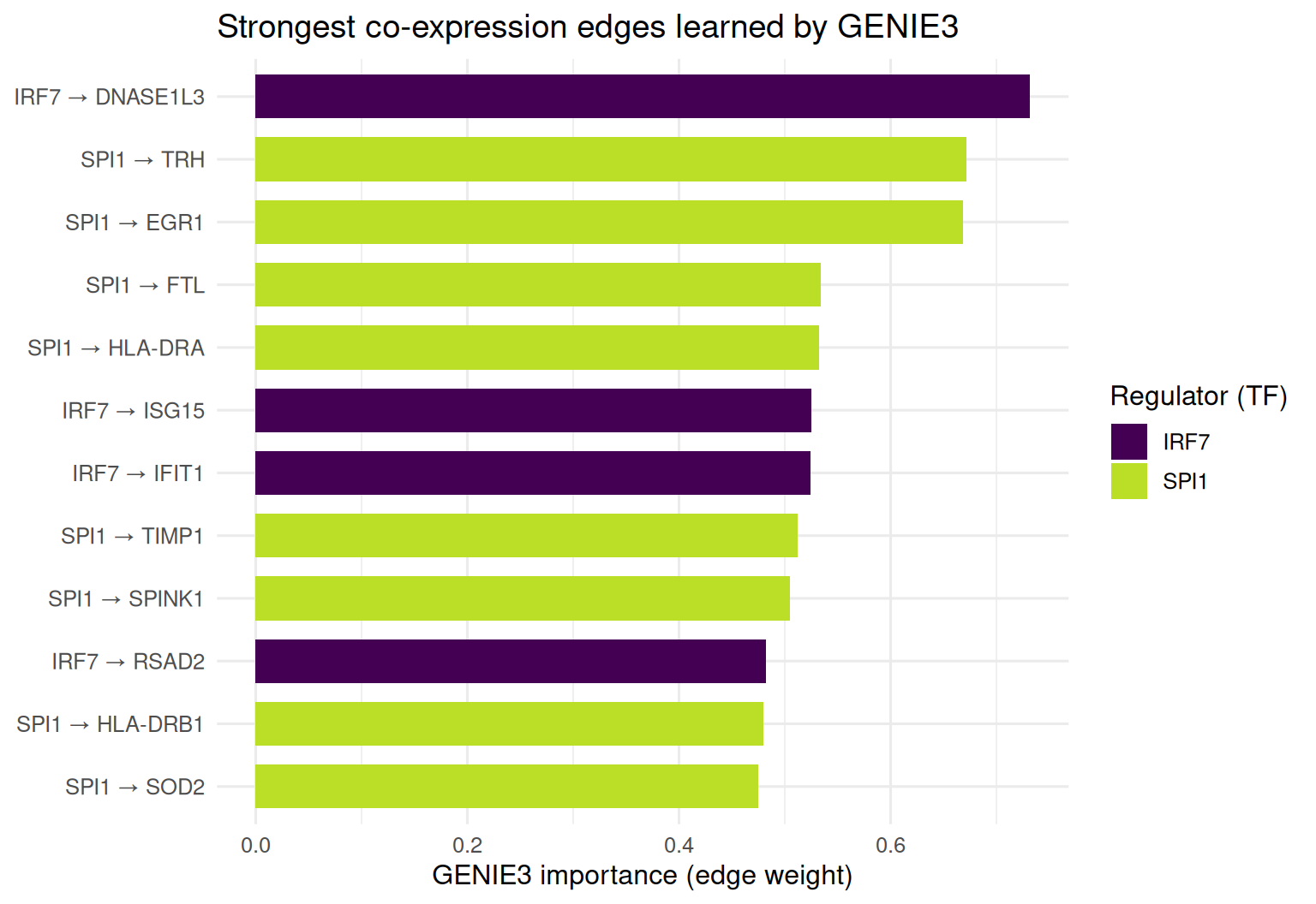
The point of the ground truth is to check the edges. Plot the strongest links GENIE3 found and read them against known immune biology.

library(ggplot2)

top <- head(lnk, 12)
top$edge <- paste(top$regulatoryGene, "→", top$targetGene)
top$edge <- factor(top$edge, levels = rev(top$edge))

ggplot(top, aes(x = edge, y = weight, fill = regulatoryGene)) +
  geom_col(width = 0.7) +
  coord_flip() +
  scale_fill_viridis_d(option = "D", end = 0.9, name = "Regulator (TF)") +
  labs(x = NULL, y = "GENIE3 importance (edge weight)",
       title = "Strongest co-expression edges learned by GENIE3") +
  theme_minimal(base_size = 12) +
  theme(legend.position = "right")

A horizontal barplot of the twelve strongest transcription-factor-to-target edges GENIE3 learned, each bar coloured by its regulator on a viridis scale. IRF7 to DNASE1L3 is the longest bar (weight about 0.73), followed by SPI1 to TRH, SPI1 to EGR1, SPI1 to FTL and SPI1 to HLA-DRA, then IRF7 to ISG15 at about 0.53. The strongest edges are split between IRF7, an interferon-regulatory factor driving interferon-stimulated genes, and SPI1 (PU.1) driving myeloid target genes — both recovered from co-expression alone.

The strongest edges split cleanly along known biology. The top link is IRF7 → DNASE1L3 (weight ≈ 0.73), and a little further down sits IRF7 → ISG15 (≈ 0.53) — a textbook interferon edge: IRF7 is a master interferon-regulatory factor, and ISG15 is one of the most induced interferon-stimulated genes in an IFN-β response. GENIE3 recovered that regulatory relationship from co-expression alone, with no prior network told to it. The other strong regulator is SPI1 (also called PU.1), a master myeloid TF, driving myeloid targets — HLA-DRA (a class-II antigen-presentation gene), FTL (ferritin light chain), EGR1. Two coherent regulatory programs — an interferon one and a myeloid one — fall straight out of the learned network. That is the promise of data-driven GRN inference: the regulons emerge from the data, not from a database.

Step 2 — RcisTarget: prune co-expression into regulons

Co-expression is necessary but not sufficient: two genes can correlate without one regulating the other (a shared upstream driver, a cell-cycle effect). SCENIC’s second step keeps only the links with a mechanistic basis. RcisTarget performs cis-regulatory motif enrichment: for each co-expression module (a TF and its GENIE3 targets), it asks whether the target genes are enriched for the TF’s binding motif near their transcription start sites, using precomputed motif-rank databases. Modules that pass become regulons — and crucially, only the direct, motif-supported targets are retained.

# Illustrative only — needs the cisTarget motif-rank databases (~1 GB feather files
# per species), so it is NOT run here. Point RcisTarget at the downloaded databases:
library(RcisTarget)

# The motif-rank databases (downloaded once from the SCENIC resources):
#   hg19-500bp-upstream-7species.mc9nr.feather, hg19-tss-centered-10kb-7species.mc9nr.feather
data(motifAnnotations_hgnc)
motifRankings <- importRankings("hg19-tss-centered-10kb-7species.mc9nr.feather")

# geneModules = the per-TF target lists distilled from the GENIE3 weight matrix above.
# RcisTarget keeps only targets carrying the TF's motif -> a pruned, direct regulon.
motifEnrichment <- cisTarget(geneModules, motifRankings,
                             motifAnnot = motifAnnotations_hgnc)

Motif pruning is what separates SCENIC from a plain co-expression network: it demands evidence that the TF can physically bind near the target, so spurious correlations are dropped and each regulon is a set of direct, sequence-supported targets (Aibar et al., 2017).

Step 3 — AUCell: score each cell for regulon activity

Once you have regulons, the final step measures how active each regulon is in each cell. SCENIC uses AUCell — the very engine taught in the gene-signature scoring lesson. For a given cell, AUCell ranks all genes by expression and computes the area under the recovery curve (AUC) for a regulon’s target genes: a cell where the regulon’s targets sit near the top of the ranking scores high. The output is a cells × regulons activity matrix you can add to your Seurat object, contrast across conditions, or paint on a UMAP — exactly as you did with curated TF activity.

# Illustrative only — runs on the regulons from step 2 (motif-pruned), which need the
# cisTarget databases. AUCell itself is light; the regulons are the gated input.
library(AUCell)

cellRankings <- AUCell_buildRankings(as.matrix(GetAssayData(obj, layer = "data")))
regulonAUC   <- AUCell_calcAUC(regulons, cellRankings)   # cells x regulons activity

# regulonAUC now scores each cell for each de-novo regulon, the same way signature
# scoring scores a curated gene set — see the AUCell / UCell lesson for the engine.

The full SCENIC pipeline

In practice you rarely wire the three steps by hand — the SCENIC package wraps them into four calls, driven by one options object. This is the real end-to-end run; it is illustrative here because every step after the first needs the motif databases.

# Illustrative only — the end-to-end SCENIC workflow. Requires the cisTarget motif
# databases and substantial compute, so it belongs in a managed environment.
library(SCENIC)

scenicOptions <- initializeScenic(org = "hgnc", dbDir = "cisTarget_databases",
                                  nCores = 8)

# 1) co-expression (GENIE3 or the faster GRNBoost2) -> TF-target modules
runGenie3(exprMat_filtered, scenicOptions)
scenicOptions <- runSCENIC_1_coexNetwork2modules(scenicOptions)

# 2) motif pruning (RcisTarget) -> regulons
scenicOptions <- runSCENIC_2_createRegulons(scenicOptions)

# 3) per-cell regulon activity (AUCell)
scenicOptions <- runSCENIC_3_scoreCells(scenicOptions, exprMat)

runSCENIC_1_coexNetwork2modules() turns the GENIE3 weight matrix into co-expression modules, runSCENIC_2_createRegulons() runs the RcisTarget motif pruning, and runSCENIC_3_scoreCells() runs AUCell — the three steps you saw individually, now orchestrated. The output is a regulon-activity matrix ready for clustering and visualisation.

Methods, honesty and reproducibility

A few things to keep straight so you use SCENIC accurately.

R SCENIC is slow and needs the cisTarget motif databases. The co-expression step scales with genes × regulators × cells, and the motif step needs roughly a gigabyte of feather databases per species. For anything beyond a demo, the Saez–Aerts-community standard is pySCENIC, the Python reimplementation, which is about tenfold faster, more memory-efficient, and containerised for reproducible runs (Van de Sande et al., 2020). The motif databases and the heavy compute belong in a managed-compute environment; this lesson runs the co-expression step and teaches the motif and scoring steps illustratively for that reason.

GRNBoost2 replaces GENIE3 for large data. pySCENIC swaps GENIE3 for GRNBoost2 — a gradient-boosting regressor that gives very similar networks in a fraction of the time (Van de Sande et al., 2020). On the small demo here GENIE3 is fine; on tens of thousands of cells and thousands of genes, GRNBoost2 is the practical choice.

De-novo regulons are noisier than curated priors — validate them. Because SCENIC learns edges statistically from this dataset, some links are spurious (the motif step removes many, not all). Treat a discovered regulon as a hypothesis: check its top targets against known biology, look for the expected regulators in a contrast you understand (here, interferon TFs in the stimulated cells), and be cautious with small or low-confidence regulons. This is the flip side of the discovery advantage — the network is dataset-specific, so it is also dataset-specific in its errors.

When to use SCENIC vs prior-based TF activity

Choose by whether the network you need already exists.

Reach for prior-based TF activity (DoRothEA/CollecTRI + decoupleR) when a curated resource covers your biology — it is fast, robust, offline, and needs no motif databases. This is the right default for standard human/mouse work.
Reach for SCENIC when the regulons that matter are specific to your data — a tumour program, a rare cell state, a non-model organism with no curated regulons — and you can afford the compute and motif databases to discover them. SCENIC finds cell-type- and condition-specific regulons the priors never encoded.
In production, prefer pySCENIC (Van de Sande et al., 2020) — the faster, containerised, GRNBoost2-based workflow — and use the R co-expression step, as here, to understand and prototype what it does.

Common issues

GENIE3 is unbearably slow (or runs out of memory) on all genes. GENIE3 trains one random forest per target gene, so cost grows with the number of genes and regulators. Never run it on the full matrix. Restrict to highly variable genes plus a candidate-TF list (as we do here), and on large data switch to GRNBoost2 via pySCENIC, which gives a similar network far faster (Van de Sande et al., 2020). Parallelise with nCores when you do run GENIE3.

RcisTarget errors that it cannot find the motif databases. Steps 2 and 3 need the cisTarget motif-rank databases — large feather files downloaded once from the SCENIC resources and pointed to with dbDir. They are not bundled with the package because of their size (~1 GB per species). Download the species-matched databases, set dbDir in initializeScenic(), and run in an environment with the disk and memory to hold them. This is why the motif and scoring steps are illustrative in a frozen lesson.

Your de-novo regulons look noisier than DoRothEA’s. They are — that is expected. SCENIC infers edges statistically from your dataset, so it captures dataset-specific regulons and dataset-specific noise. Validate against known biology (do the interferon TFs surface in the stimulated cells?), keep higher-confidence regulons, and if you only need a vetted network for standard biology, prior-based TF activity is the more robust choice.

Frequently asked questions

SCENIC vs DoRothEA/CollecTRI — what is the difference?

Both give you transcription-factor regulons, but from opposite directions. DoRothEA/CollecTRI are curated regulon databases built once from literature and evidence — fast, robust, offline, and limited to what curators encoded. SCENIC learns regulons de novo from your dataset with GENIE3 co-expression plus RcisTarget motif pruning, so it can discover cell-type- and condition-specific regulons the priors never had — at the cost of compute, motif databases, and noisier edges. Use curated priors when they cover your biology; use SCENIC to discover regulons specific to your data.

Can I run SCENIC fully in R?

Yes, with the R SCENIC package plus GENIE3, RcisTarget and AUCell — but only the GENIE3 co-expression step is light. The motif step needs the cisTarget databases (~1 GB per species) and the whole pipeline is slow. For anything beyond a prototype, the community standard is pySCENIC, the Python reimplementation, which is roughly tenfold faster and containerised (Van de Sande et al., 2020). A common pattern is to prototype and learn the steps in R, then run production in pySCENIC.

GENIE3 vs GRNBoost2 — which co-expression method should I use?

Both infer the same kind of co-expression network — how well each TF predicts each target — but with different regressors. GENIE3 uses random forests (Huynh-Thu et al., 2010) and is the original SCENIC engine; GRNBoost2 uses gradient boosting and gives very similar networks much faster, which is why pySCENIC adopts it for large datasets (Van de Sande et al., 2020). For a small demo, GENIE3 is fine; for tens of thousands of cells, prefer GRNBoost2.

Why does SCENIC need motif databases at all — isn’t co-expression enough?

Co-expression alone confuses correlation with regulation: two genes can move together because of a shared upstream driver, the cell cycle, or a batch effect, without one controlling the other. SCENIC’s RcisTarget step demands mechanistic evidence — it keeps only targets that carry the TF’s binding motif near their promoter — so each regulon is a set of direct, sequence-supported targets rather than mere co-expression partners (Aibar et al., 2017). That pruning is what makes SCENIC’s regulons trustworthy, and it is why the motif databases are required.

How is AUCell here different from AUCell in the signature-scoring lesson?

It is the same tool doing the same job — scoring each cell for a gene set by ranking its genes and taking the area under the recovery curve. The only difference is what gene set it scores: in signature scoring you supply a curated list; in SCENIC the gene sets are the regulons SCENIC just learned and motif-pruned. Once you have regulons, per-cell scoring is identical to signature scoring.

Test your understanding

Your turn: read the learned network for a myeloid regulator

Using ifnb_subset.rds, build the GENIE3 co-expression network as in this lesson (HVGs + the candidate-TF list, 400 cells, set.seed(42)). From the ranked edge list, pull out only the edges whose regulator is SPI1 and look at its top targets. Are they myeloid genes — the kind of program PU.1/SPI1 is known to drive?

Hint

After lnk <- getLinkList(wm), subset with lnk[lnk$regulatoryGene == "SPI1", ] and take head(...). The getLinkList output already comes ranked by weight, so the first rows are SPI1’s strongest targets.

Solution

library(Seurat); library(GENIE3)
d   <- readRDS("_data/ifnb_subset.rds")
obj <- NormalizeData(CreateSeuratObject(counts = d$counts, meta.data = d$meta))
obj <- FindVariableFeatures(obj, nfeatures = 200)
hvg <- head(VariableFeatures(obj), 120)
tfs <- intersect(c("STAT1", "STAT2", "IRF1", "IRF7", "IRF9", "NFKB1",
                   "REL", "SPI1", "CEBPB", "FOS", "JUN", "EGR1"), rownames(obj))
set.seed(42)
cells <- sample(colnames(obj), 400)
expr  <- as.matrix(GetAssayData(obj, layer = "data")[union(hvg, tfs), cells])
set.seed(42)
wm  <- GENIE3(expr, regulators = tfs, nCores = 1)
lnk <- getLinkList(wm)

# SPI1's strongest learned targets
head(lnk[lnk$regulatoryGene == "SPI1", ])

SPI1’s top targets include EGR1, FTL and HLA-DRA — myeloid and antigen-presentation genes, exactly the kind of program the master myeloid TF PU.1/SPI1 drives — alongside noisier data-driven links such as TRH that are not canonical SPI1 targets, a reminder that de-novo edges need validation. GENIE3 still recovered a largely coherent SPI1 program from co-expression alone, alongside the interferon (IRF7) program — two dataset-specific regulatory modules, learned without any prior network.

Quick check: SCENIC’s GENIE3 step ranks IRF7 → ISG15 as a strong edge. What does that edge actually mean, and why is it reassuring here?

A. It means ISG15’s promoter was experimentally shown to bind IRF7 in these cells. B. It means IRF7’s expression predicts ISG15’s expression well across cells (a co-expression link) — a plausible regulatory edge that GENIE3 learned from the data, and reassuring because IRF7 is an interferon regulator and ISG15 an interferon-stimulated gene, so the biology is exactly right for an IFN-β dataset. C. It means ISG15 is a transcription factor that regulates IRF7.

Show answer

B. GENIE3’s edge weight is a co-expression / predictive-importance score: IRF7’s expression is a good predictor of ISG15’s across cells, so GENIE3 proposes a regulatory link. It is not direct binding evidence — that is exactly what SCENIC’s step 2 (RcisTarget motif pruning) adds. The edge is reassuring because IRF7 is a master interferon-regulatory factor and ISG15 a canonical interferon-stimulated gene, so recovering this link from an IFN-β dataset shows the learned network is tracking real biology. (A overclaims — GENIE3 has no binding data; C reverses the roles — IRF7 is the TF, ISG15 the target.)

Conclusion

SCENIC infers a gene regulatory network de novo from your own single-cell data rather than scoring a curated one. Its three steps narrow a broad, noisy signal into trustworthy regulons: GENIE3 learns a co-expression network by random-forest importance, RcisTarget prunes it to motif-supported targets, and AUCell scores each cell for each regulon’s activity. Here the GENIE3 step ran end to end and recovered coherent biology from co-expression alone — the interferon edge IRF7 → ISG15 and a myeloid SPI1 program — while the motif and scoring steps, which need the cisTarget databases, were shown illustratively; in production, pySCENIC with GRNBoost2 is the faster, scalable standard.

This closes the functional-inference toolkit for single-cell RNA-seq. You now have four complementary ways to ask what cells are doing: gene-signature scoring asks does a cell express this gene set?; pathway activity asks is a signaling pathway firing?; prior-based TF activity asks which curated regulator is active?; and data-driven GRN inference asks what regulatory network does this dataset reveal on its own? Curated when a resource covers your biology, data-driven when it does not — together they take you from a gene list to the regulatory logic of your cells.

References

Aibar, S., González-Blas, C. B., Moerman, T., Huynh-Thu, V. A., Imrichova, H., Hulselmans, G., Rambow, F., Marine, J.-C., Geurts, P., Aerts, J., van den Oord, J., Atak, Z. K., Wouters, J., & Aerts, S. (2017). SCENIC: single-cell regulatory network inference and clustering. Nature Methods, 14(11), 1083–1086. https://doi.org/10.1038/nmeth.4463
Van de Sande, B., Flerin, C., Davie, K., De Waegeneer, M., Hulselmans, G., Aibar, S., Seurinck, R., Saelens, W., Cannoodt, R., Rouchon, Q., Verbeiren, T., De Maeyer, D., Reumers, J., Saeys, Y., & Aerts, S. (2020). A scalable SCENIC workflow for single-cell gene regulatory network analysis — introduces pySCENIC and GRNBoost2. Nature Protocols, 15(7), 2247–2276. https://doi.org/10.1038/s41596-020-0336-2
Huynh-Thu, V. A., Irrthum, A., Wehenkel, L., & Geurts, P. (2010). Inferring regulatory networks from expression data using tree-based methods — introduces GENIE3. PLoS ONE, 5(9), e12776. https://doi.org/10.1371/journal.pone.0012776
Kang, H. M., et al. (2018). Multiplexed droplet single-cell RNA-sequencing using natural genetic variation — the source of the IFN-β–stimulated PBMC dataset. Nature Biotechnology, 36, 89–94. https://doi.org/10.1038/nbt.4042

Reuse

CC BY-NC-SA 4.0

Citation

BibTeX citation:

@online{2026,
  author = {},
  title = {Gene {Regulatory} {Network} {Inference} in {R:} {GENIE3} \&
    {SCENIC} for {Single-Cell} {RNA-Seq}},
  date = {2026-07-04},
  url = {https://www.datanovia.com/learn/bioinformatics/single-cell/scrnaseq-gene-regulatory-networks-scenic.html},
  langid = {en}
}

For attribution, please cite this work as:

“Gene Regulatory Network Inference in R: GENIE3 & SCENIC for Single-Cell RNA-Seq.” 2026. July 4. https://www.datanovia.com/learn/bioinformatics/single-cell/scrnaseq-gene-regulatory-networks-scenic.html.