Aggregate, read, and plot FASTQC reports for many samples with the fastqcr package
Bioinformatics
Quality-control raw sequencing reads in R with the fastqcr package — aggregate FASTQC reports across many samples, read per-module results, plot each quality metric, and flag failures and warnings. A reproducible QC workflow for high-throughput sequencing data.
Published
July 8, 2026
Modified
July 9, 2026
TipKey takeaways
FastQC is the standard tool for QC (quality control) of raw sequencing reads; it emits one HTML report and a .zip of raw metrics per sample. With hundreds of samples, you cannot open each by hand — you need to read them in aggregate.
fastqcr (an R package we maintain — install.packages("fastqcr")) parses those .zip outputs and turns them into tidy data frames you analyze in R: aggregate across samples, summarize, flag problems, read per-module results, and plot each metric.
qc_aggregate() walks a directory of FASTQC outputs and returns one long data frame: sample × module × status plus read count, read length, %GC, and %duplicates.
qc_fails() / qc_warns() / qc_problems() answer the two questions that matter: which modules failed across the most samples? and which samples are the worst?
qc_read() loads one sample’s raw metrics (14 elements) and qc_plot() draws any module — per-base quality, GC content, duplication, adapter content — so you can see why a flag was raised.
library(fastqcr)# One sample's FASTQC report, bundled with the package:qc.file <-system.file("fastqc_results", "S1_fastqc.zip", package ="fastqcr")s1 <-qc_read(qc.file) # read all modules for this sampleqc_plot(s1, "Per base sequence quality") # the figure everyone recognizes
The most-recognized FastQC figure: read quality across positions. The green band is good quality, orange reasonable, red poor — this sample stays in the green the whole way. That is what fastqcr gives you for every sample and every module. We come back to reading each one below; first, the workflow that gets you there.
Introduction
You have just received raw sequencing data — an RNA-seq run, an exome, a genome — and the folder holds one .fastq.gz per sample containing millions of short reads. Before you align or count anything, you need to know whether the raw reads are any good: are the base qualities high, is there adapter contamination, is the duplication level alarming? That check is quality control (QC), and the tool everyone uses for it is FastQC, a quality-control program for high-throughput sequencing reads written by Simon Andrews at the Babraham Institute.
FastQC runs a series of tests (called analysis modules) on each sample and writes an HTML report plus a .zip of the underlying numbers. That is perfect for one or two samples and unmanageable for a hundred — you are not going to click through a hundred HTML pages. This is exactly the gap fastqcr fills: it is an R package (one we maintain) that reads FastQC’s .zip outputs into tidy data frames so you can aggregate, summarize, inspect, and plot many samples at once — and build a single multi-sample QC report. This lesson takes you through that workflow on the example reports bundled with the package, so every result here is reproducible on your own machine.
The fastqcr workflow
fastqcr does not replace FastQC — it reads what FastQC produced and makes it analyzable in R. The main functions group into a short pipeline: run (or point at existing) FastQC output, aggregate it, inspect problems, then read and plot individual samples.
The main functions of the fastqcr package: run FastQC (fastqc_install, fastqc), aggregate and summarize reports (qc_aggregate, summary, qc_stats), inspect problems (qc_fails, qc_warns, qc_problems), import and plot (qc_read, qc_plot), and build HTML reports (qc_report).
The rest of this lesson works through those stages in order.
Install and load fastqcr
fastqcr is on CRAN — a plain install.packages(), no Bioconductor or Docker needed:
if (!require(devtools)) install.packages("devtools")devtools::install_github("kassambara/fastqcr")
Then load it:
library(fastqcr)
Aggregate FASTQC reports across samples
The workhorse is qc_aggregate(). Point it at a directory of FastQC outputs and it walks every zipped result folder, reads the fastqc_data.txt (raw metrics) and summary.txt (per-module status) inside each, and returns one long data frame — the whole run in a single object you can filter and summarize.
The package ships a demo directory of five samples so you can run this without your own data:
# Demo FASTQC output directory bundled with fastqcr:qc.dir <-system.file("fastqc_results", package ="fastqcr")list.files(qc.dir) # five zipped FASTQC reports, S1–S5
Read down the nb_fail / nb_warn columns: Per base sequence content fails in all 5 samples, Per sequence GC content fails in 2 (S3, S4) and warns in 3 (S1, S2, S5), and Sequence Length Distribution warns in all 5. Every other module passes cleanly. That is your triage list — three modules to understand, nine you can set aside.
General statistics per sample
qc_stats() collapses the run to one row per sample with the headline numbers:
The five samples carry 50–67 million reads each, read lengths of 35–76 bp, ~48–49% GC, and 16–22% duplicates — consistent across samples, which is what a well-behaved run looks like. A single sample with wildly different GC or duplication would jump out here immediately.
Inspect problems
For triage you want the two views directly: which modules are worst across samples? and which samples are worst overall? Three functions provide them — qc_fails() (failures only), qc_warns() (warnings only), and qc_problems() (their union). Each takes an element argument, "module" or "sample".
Which modules failed the most?
qc_fails(qc, "module")
# A tibble: 2 × 3
  module                    nb_problems sample
  <chr>                           <int> <chr>
1 Per base sequence content           5 S1, S2, S3, S4, S5
2 Per sequence GC content             2 S3, S4
Per base sequence content failed in all 5 samples and Per sequence GC content in 2 — the same two modules the summary flagged, now ranked by how widespread the failure is. The compact output lists, per module, the number of failures and the samples responsible.
To zoom in on a single module across all its samples, name it (partial matching works, so "GC content" finds "Per sequence GC content"):
qc_problems(qc, "module", name ="Per sequence GC content")
# A tibble: 5 × 4
  module                  nb_problems sample status
  <chr>                         <int> <chr>  <chr>
1 Per sequence GC content           5 S3     FAIL
2 Per sequence GC content           5 S4     FAIL
3 Per sequence GC content           5 S1     WARN
4 Per sequence GC content           5 S2     WARN
5 Per sequence GC content           5 S5     WARN
Which samples are worst?
Flip element to "sample" to rank samples instead of modules:
qc_fails(qc, "sample")
# A tibble: 5 × 3
  sample nb_problems module
  <chr>        <int> <chr>
1 S3               2 Per base sequence content, Per sequence GC content
2 S4               2 Per base sequence content, Per sequence GC content
3 S1               1 Per base sequence content
4 S2               1 Per base sequence content
5 S5               1 Per base sequence content
S3 and S4 each carry two failed modules; S1, S2, and S5 one apiece — so S3 and S4 are the samples to scrutinize first. For each sample the output gives the number of problems and names the modules that failed.
Read one sample into R
Aggregation gives you the run-level picture; to see why a module was flagged you read one sample’s raw metrics with qc_read(), which returns a named list of data frames — one per module:
qc.file <-system.file("fastqc_results", "S1_fastqc.zip", package ="fastqcr")s1 <-qc_read(qc.file)length(s1) # number of elements
[1] 14
names(s1) # one per FastQC module (+ the summary and basic stats)
Fourteen elements: the 12 analysis modules plus the overall summary and the total_deduplicated_percentage. Each element is a tidy data frame you could inspect directly — but the fastest way to read a module is to plot it.
Plot and interpret each module
qc_plot() draws any module from a qc_read() object. The plots below are FastQC’s standard figures, rendered from R — and the interpretation prose is the real payoff: knowing what each module measures and when a flag actually matters. The authoritative definitions live in the FastQC analysis-modules documentation.
Per base sequence quality
The quality score across all reads at each base position — the figure at the top of this lesson. The background bands mark quality zones: green (good), orange (reasonable), red (poor); a good sample sits entirely in the green, as S1 does. FastQC raises a warning if the median quality at any position drops below 25, a failure below 20. Quality that decays toward the 3′ end is the classic pattern you fix with quality trimming before alignment.
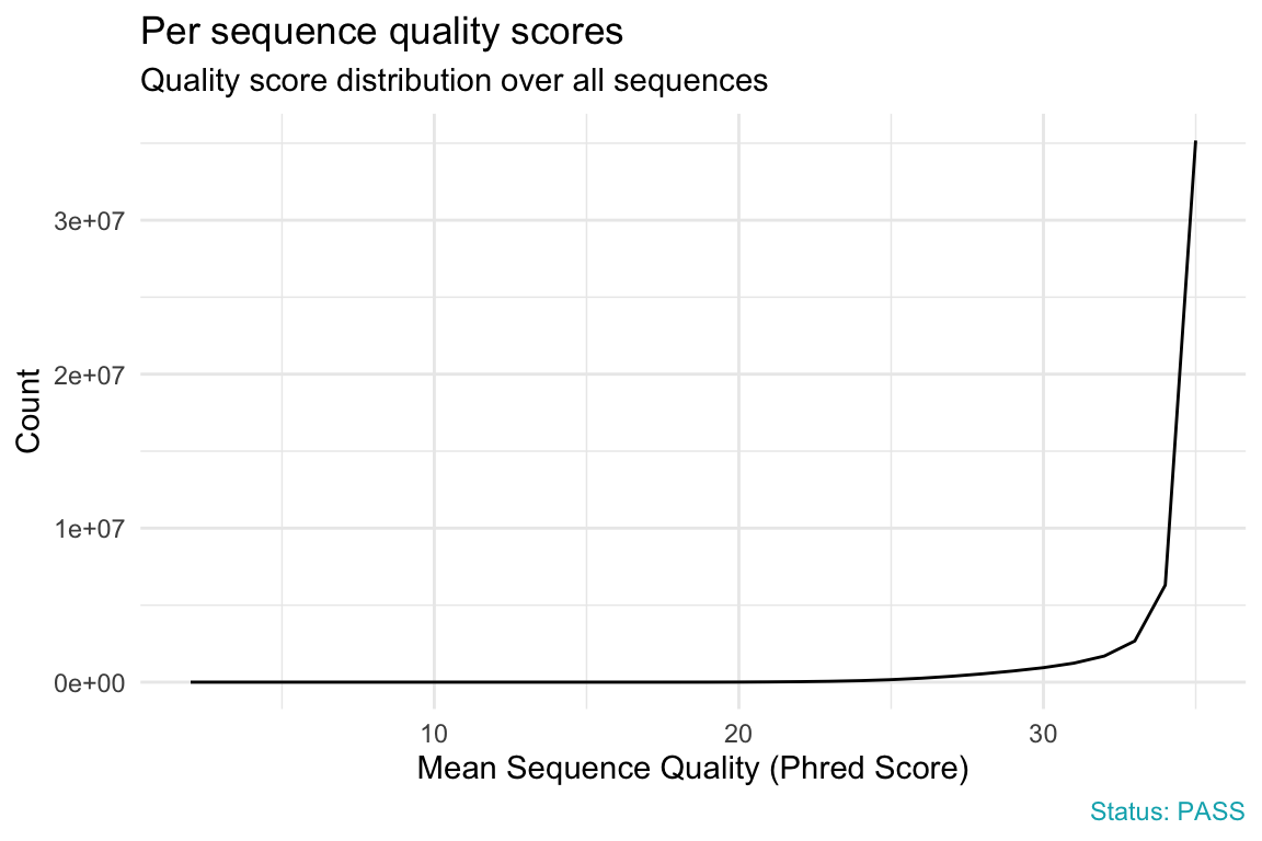
Per sequence quality scores
The distribution of mean quality per read. It reveals whether a subset of reads is uniformly poor. A good library peaks far to the right (mean quality > 27).
qc_plot(s1, "Per sequence quality scores")
A warning fires if the most common mean quality is below 27 (a 0.2% error rate), a failure below 20 (a 1% error rate). A left-shifted peak means a general loss of quality across the run.
Per base sequence content
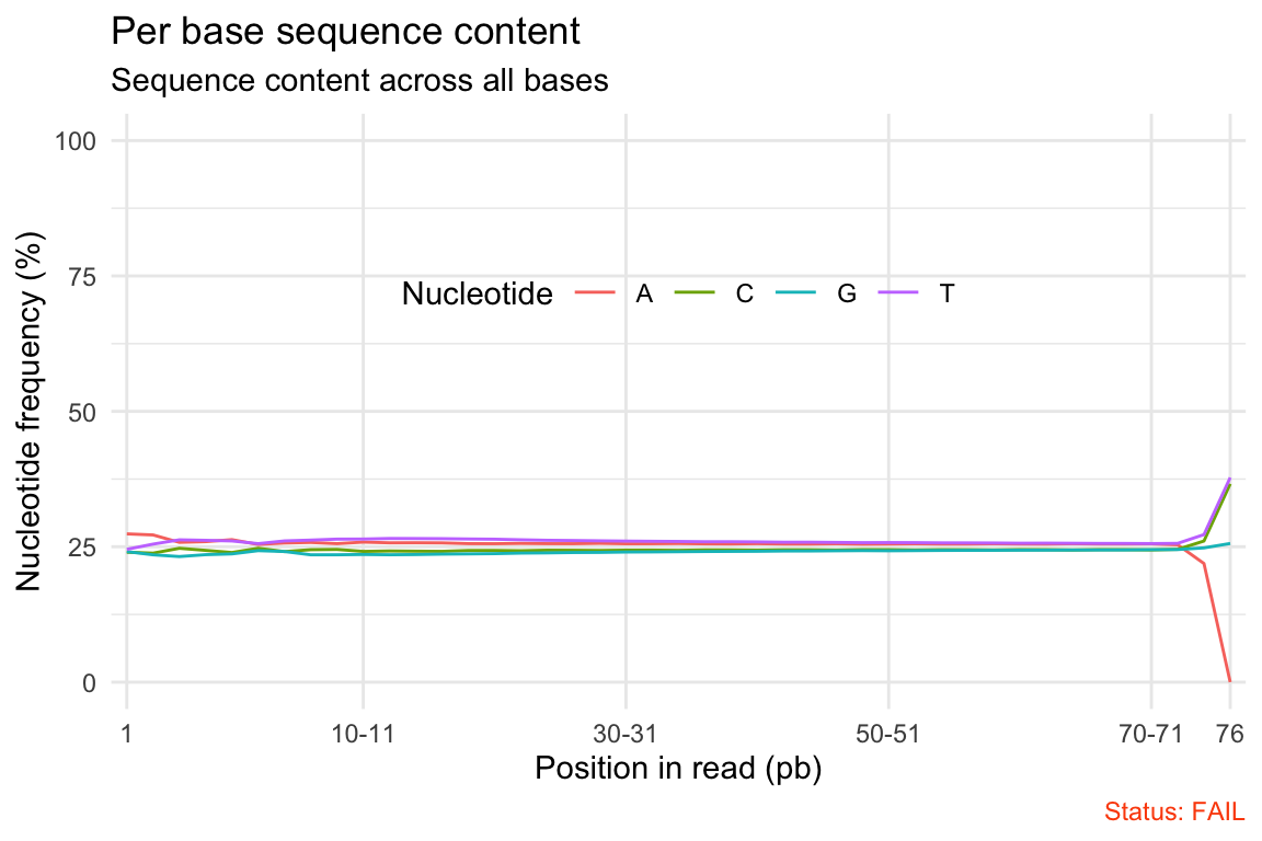
The proportion of A, C, G, and T at each position. In a random library the four lines run roughly parallel; a large gap between them signals biased composition.
qc_plot(s1, "Per base sequence content")
FastQC fails this module for the demo sample — but read why before you worry. Across almost the whole read the four nucleotide lines run flat and parallel (composition is even; the A–T spread stays under the 10% warning threshold). The failure is driven by a sharp divergence at the final base: A collapses toward 0% while T and C jump to roughly 37%. That end-of-read spike is an adapter read-through / end-of-read base-calling artifact — it disappears once you trim adapters and low-quality read ends.
The other classic cause of this module failing is RNA-seq random priming: the “random” hexamers used in library prep are not truly random and bias the composition of the first ~10–12 bases, so nearly every RNA-seq library fails here. That is a well-known library-prep signature, not a data problem, and it does not affect expression estimates. So a “Per base sequence content” fail is usually explained by one of these two — an end-of-read/adapter artifact or RNA-seq priming bias — rather than a genuinely bad library.
Per sequence GC content
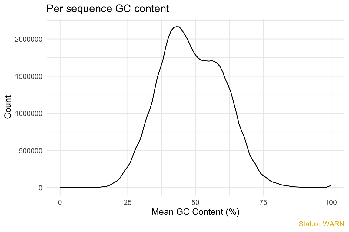
The GC distribution across reads. A random library gives a roughly normal curve centered on the genome’s GC; a sharp or shifted peak hints at contamination or a systematic bias.
qc_plot(s1, "Per sequence GC content")
A warning means the observed distribution deviates modestly from the theoretical normal (as here); a failure means a large departure. A secondary peak often indicates a contaminant or an over-represented sequence.
Per base N content
The percentage of bases the sequencer could not call (reported as N) at each position. It should sit near zero everywhere.
qc_plot(s1, "Per base N content")
A warning fires above 5% at any position, a failure above 20%. A spike usually accompanies a general loss of quality or a strongly biased composition.
Sequence length distribution
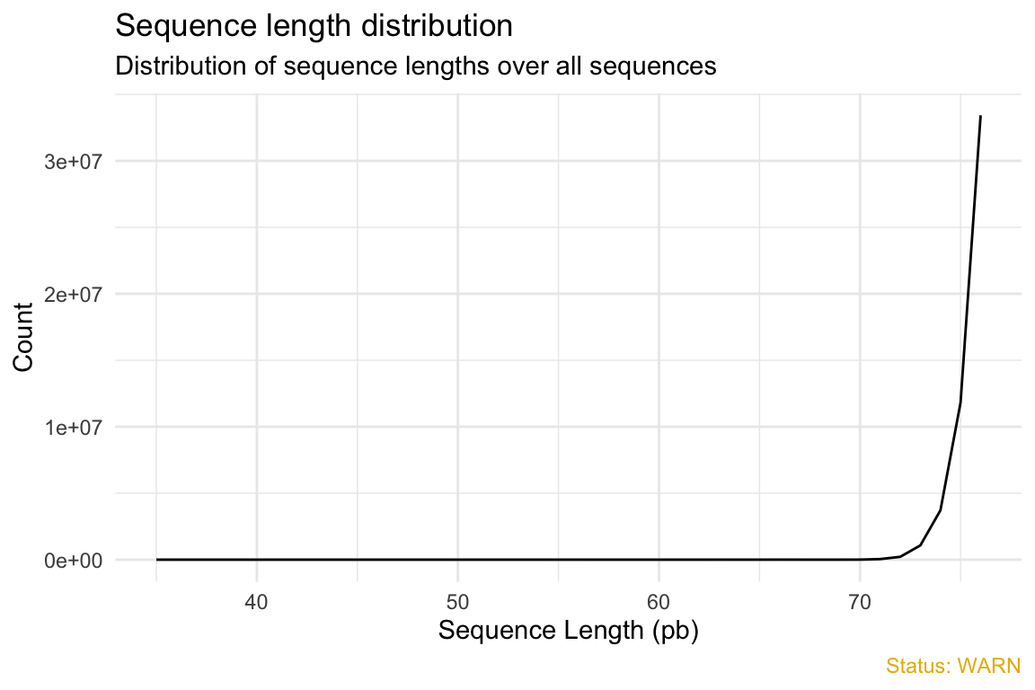
Whether all reads share one length. Many platforms produce a single length (one peak); others legitimately vary, so a warning here is often benign.
qc_plot(s1, "Sequence length distribution")
These reads span 35–76 bp, so FastQC warns — but variable length is normal after adapter trimming, so this flag can be ignored. The module only truly errors if any read has zero length.
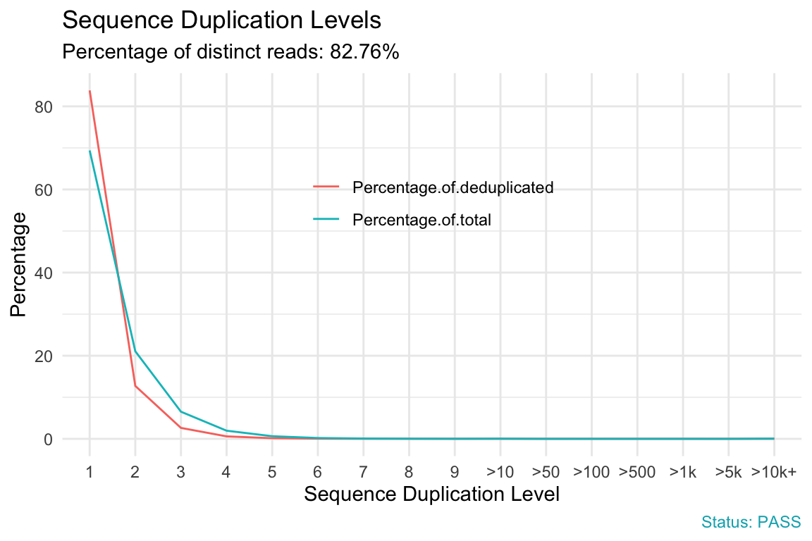
Sequence duplication levels
The degree of duplication across reads. High duplication can indicate enrichment bias such as PCR over-amplification.
qc_plot(s1, "Sequence duplication levels")
A warning fires when non-unique reads exceed 20% of the total, a failure above 50%. In RNA-seq, duplication of 20–40% is normal — highly expressed genes genuinely produce identical reads — so you should not blindly deduplicate transcriptome data; a duplicate may be biology, not a PCR artifact.
Overrepresented sequences
Any single sequence making up more than 0.1% of the library — a signal of adapter, primer, or rRNA contamination, or simply low library diversity.
qc_plot(s1, "Overrepresented sequences")
A warning fires when any sequence exceeds 0.1% of reads, a failure above 1%. Small-RNA libraries naturally trigger this and can be an exception.
Adapter content
The cumulative fraction of reads containing known adapter sequences at each position. It tells you whether adapter trimming is needed before downstream analysis.
qc_plot(s1, "Adapter content")
A warning fires when adapter is present in more than 5% of reads at any position, a failure above 10%. A flag here means you should adapter-trim before aligning.
Build an HTML QC report
Beyond interactive analysis, qc_report() writes a shareable HTML report — either a multi-sample report from a directory, or a one-sample report with plot interpretations built in. Point it at the demo directory:
# Multi-sample report from a directory of FASTQC outputs:qc_report(qc.dir, result.file ="multi-qc-report",experiment ="Exome sequencing of colon cancer cell lines")
# One-sample report, with the per-module interpretations included:qc.file <-system.file("fastqc_results", "S1_fastqc.zip", package ="fastqcr")qc_report(qc.file, result.file ="one-sample-report", interpret =TRUE)
These are shown as illustrative calls (not run here) because they write files to disk; run them locally to produce the reports.
Running FastQC itself
If you do not yet have FastQC output, fastqcr can install and run the FastQC tool for you on macOS/Linux — fastqc_install() fetches the latest release, and fastqc() runs it over a directory of FASTQ files:
fastqc_install() # install the FastQC tool (macOS / Linux)fastqc(fq.dir ="~/Documents/FASTQ", # directory of .fastq(.gz) filesqc.dir ="~/Documents/FASTQC", # where to write the reportsthreads =4)
FastQC accepts FASTQ and gzip-compressed FASTQ. Once it has written its .zip outputs, you are back at the top of this workflow with qc_aggregate().
Common issues
qc_aggregate() returns an empty or partial data frame. It expects the zipped FastQC output folders (*_fastqc.zip) as FastQC writes them — point qc.dir at the directory that contains those .zip files, not at an unzipped folder or the FASTQ files. If you unzipped them, qc_unzip() and the directory of unzipped folders also work.
All demo samples fail “Per base sequence content” — usually not a real defect. For these reports the failure comes from an end-of-read/adapter artifact at the last base, cleared by trimming. In RNA-seq data the same module fails almost universally for a different reason — random-priming bias over the first ~10–12 bases — which is likewise a known library-prep signature, not a data problem, and does not affect expression quantification.
A warning looks alarming but is benign. FastQC’s thresholds are generic; a library type can legitimately trip a module (variable read length after trimming, high duplication from highly expressed genes, biased composition in bisulphite libraries). Treat WARN/FAIL as “look here”, not “discard the sample” — read the module and decide in context.
Frequently asked questions
NoteWhat is FastQC, and what does fastqcr add?
FastQC is a quality-control tool for high-throughput sequencing reads: it runs a set of analysis modules on each sample and writes an HTML report plus a .zip of raw metrics. fastqcr is an R package that reads those .zip outputs into tidy data frames so you can aggregate, summarize, inspect, and plot many samples at once in R — and build a single multi-sample report — instead of clicking through one HTML page per sample.
NoteHow do I aggregate FastQC reports for many samples in R?
Point qc_aggregate() at the directory holding the zipped FastQC outputs: qc <- qc_aggregate("path/to/fastqc_results"). It returns one long data frame with a row per sample × module, carrying the status and the general statistics (reads, length, %GC, %duplicates). From there, summary(qc), qc_stats(qc), and qc_fails(qc, "module") summarize the whole run.
NoteWhat do PASS, WARN, and FAIL mean in FastQC?
They are FastQC’s per-module verdicts against fixed thresholds: PASS = normal, WARN = slightly unusual, FAIL = very unusual. They are pointers, not a pass/fail grade for the sample — some library types are expected to trip specific modules (e.g. RNA-seq fails per-base sequence content). Always read the flagged module in context before acting.
NoteShould I remove duplicate reads in RNA-seq?
Usually no. RNA-seq duplication of 20–40% is normal because highly expressed genes genuinely produce identical reads, so you cannot tell a PCR duplicate from real high expression. FastQC may warn or fail the duplication module, but blindly deduplicating transcriptome data removes signal. Deduplication makes more sense for DNA applications with UMIs.
NoteWhy does “Per base sequence content” so often fail?
Two common causes, both benign. End-of-read / adapter artifacts skew the composition of the last base(s) — that is what fails the module for the demo reports here — and go away once you trim adapters and low-quality ends. Separately, RNA-seq random priming biases the first ~10–12 bases because the “random” hexamers used in library prep are not truly random; this trips the module for nearly all RNA-seq libraries. Neither is a fixable defect nor affects expression measurement, so both are usually safe to note and move on.
Test your understanding
ImportantYour turn: rank the run’s problems both ways
Using the bundled demo directory, aggregate the five FastQC reports and answer two questions: (1) which module failed in the most samples, and (2) which sample has the most failed modules?
TipHint
Aggregate with qc_aggregate(), then call qc_fails() twice — once with element = "module" and once with element = "sample".
TipSolution
library(fastqcr)qc.dir <-system.file("fastqc_results", package ="fastqcr")qc <-qc_aggregate(qc.dir, progressbar =FALSE)qc_fails(qc, "module") # (1) Per base sequence content — failed in all 5 samplesqc_fails(qc, "sample") # (2) S3 and S4 — two failed modules each
Per base sequence content is the most widespread failure (all 5 samples — the RNA-seq priming bias), and S3 / S4 are the worst samples with two failed modules each. Neither is a reason to discard data here; both are read in context.
NoteQuick check: a module shows FAIL — which flag is expected and benign for RNA-seq?
A. Per base sequence quality B. Per base sequence content C. Adapter content
TipShow answer
B.Per base sequence content fails for almost every RNA-seq library because random-priming biases the first bases of each read — it is expected and does not affect expression estimates. A failing per base sequence quality (poor Phred scores) or adapter content (contamination) is a real problem you would act on with trimming.
Conclusion
You ran a complete sequencing-QC workflow in R: qc_aggregate() turned a directory of FastQC outputs into one analyzable data frame, summary() and qc_stats() summarized the run per module and per sample, and qc_fails() / qc_warns() / qc_problems() ranked the problems both ways. Then qc_read() and qc_plot() let you open a single sample and read each module’s figure — and, crucially, decide whether a flag matters (an RNA-seq per-base-content failure is expected; poor base quality or adapter contamination is not). With QC done, the reads are ready for alignment and quantification into a count matrix.
This lesson is reproducible: every table and figure on this page was produced by the code shown, on the example reports bundled with fastqcr — copy any block and run it to reproduce these results. The runtime is the judge.
References
Kassambara, A. (2019). fastqcr: Quality Control of Sequencing Data — R package, CRAN · GitHub.
Andrews, S. FastQC: A Quality Control Tool for High Throughput Sequence Data — Babraham Bioinformatics.