Per-Cell Transcription Factor Activity in R with decoupleR & DoRothEA

Go one level deeper than pathway activity: infer which transcription factors are active in each cell from the expression of their regulon — the target genes they control — with DoRothEA regulons and decoupleR, validated against a known interferon response

A practical guide to per-cell transcription-factor (TF) activity for single-cell RNA-seq in R. Use the DoRothEA regulons with decoupleR’s univariate linear model (run_ulm) to infer the activity of hundreds of TFs in every cell from their target genes, contrast them across an interferon-beta stimulation, and validate the result against the built-in ground truth — IFN-beta drives the ISGF3 complex (STAT1, STAT2, IRF9) and the IRF family, so those TFs’ activity must explode in the stimulated cells. Includes how TF activity differs from pathway activity and gene-signature scoring, and DoRothEA vs the newer CollecTRI.

TipKey takeaways

• Transcription-factor activity is read from a TF’s regulon, not its own mRNA. A transcription factor (TF — a protein that switches genes on or off) is often expressed at a flat, low level even when it is driving a huge response. What moves is the coordinated expression of the genes it controls — its regulon. Inferring TF activity means reading the regulon, not the TF’s own transcript.
• DoRothEA supplies the regulons; decoupleR scores them per cell. DoRothEA (a curated collection of TF-to-target regulons with confidence tiers A–E and a signed mode of regulation) provides which genes each TF regulates (Garcia-Alonso et al., 2019); decoupleR runs that network against every cell to return a per-cell activity score for each TF (Badia-i-Mompel et al., 2022).
• run_ulm is the recommended default — a univariate linear model. It regresses each cell’s expression on a TF’s signed target weights, and the fitted slope (its t-value) becomes that TF’s activity. decoupleR also offers run_mlm, run_wsum and a consensus, but run_ulm is the documented default for TF activity.
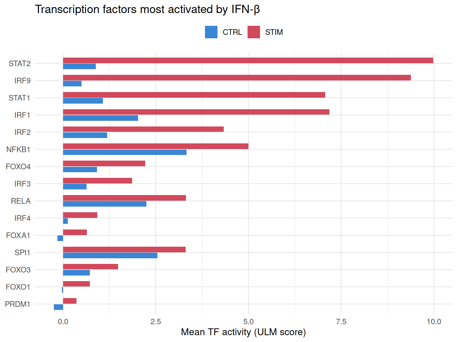
• Validate against a known contrast. Half the cells were stimulated with interferon-beta (IFN-β), which activates the JAK-STAT axis and its transcription factors. The TFs whose activity jumps most between control and stimulated cells are STAT2, IRF9, STAT1 and IRF1 — the ISGF3 complex (STAT1 + STAT2 + IRF9) and the interferon-regulatory-factor family, the canonical type-I interferon TFs. The regulons recover the biology from target genes alone.
• This completes the functional-inference trilogy. Signature scoring asks does a cell express this gene set?; pathway activity asks is a signaling pathway firing?; TF activity asks which transcription factor is driving the program? — three complementary levels of the same functional question.

Introduction

You have run the standard single-cell RNA-seq (scRNA-seq — RNA sequencing one cell at a time) workflow: quality control, clustering, cell-type annotation. You have started to quantify what cells are doing — you may have scored gene signatures and inferred which signaling pathways are firing. The next question is sharper still: which transcription factors are driving the response? A pathway tells you the signal is on; the transcription factors are the machinery that actually rewrites the cell’s gene-expression program.

Here is the catch that makes TF activity worth inferring rather than just reading off. A transcription factor’s own mRNA is a poor readout of its activity. STAT1 can be sitting at a low, flat expression level and yet, once phosphorylated by interferon signaling, switch on hundreds of genes. Its activity is invisible in its own transcript — but it is written all over the genes it controls. That set of controlled genes is the TF’s regulon, and inferring TF activity means reading the coordinated expression of the regulon back to a single per-cell activity score.

This lesson builds per-cell TF activity with two tools from the Saez-Rodriguez lab: DoRothEA (a curated collection of TF regulons) supplies which genes each TF regulates, and decoupleR scores that network in every cell. We work on the classic IFN-β immune-PBMC benchmark: peripheral blood mononuclear cells (PBMCs — the immune cells in blood) split into a control group and a group stimulated with interferon-beta (IFN-β) (Kang et al., 2018). IFN-β signals through the JAK-STAT axis to activate the ISGF3 complex — a trimer of the transcription factors STAT1, STAT2 and IRF9 — and the interferon-regulatory-factor (IRF) family. That hands us a built-in ground truth: those TFs’ activity must be far higher in the stimulated cells. If the regulons cannot recover a signal that strong, we should not trust them on a subtle one.

Three levels of functional inference: which question are you asking?

TF activity is the third of three related-but-distinct functional questions. It is worth being precise about how they differ, because they are easy to conflate and answer genuinely different things.

	Signature scoring	Pathway activity	Transcription-factor activity
Question	Does this cell express this gene set?	Is this signaling pathway firing?	Which transcription factor is active?
Genes read	The set’s own members	A pathway’s downstream response genes	A TF’s regulon — the genes it regulates
Resource	Your curated list	PROGENy (~14 pathways)	DoRothEA / CollecTRI (hundreds of TFs)
Granularity	One program	A handful of signaling pathways	Individual regulators, hundreds of them
Tool	AUCell, UCell	PROGENy + decoupleR	DoRothEA + decoupleR (this lesson)

Signature scoring asks about membership — how enriched a cell is for the genes in a set. Pathway activity and TF activity are both footprint models: they infer a regulator’s activity from the genes it leaves a mark on downstream, not from the regulator’s own expression. The difference between the two is resolution. Pathway activity with PROGENy summarises the transcriptome into about fourteen broad signaling pathways — JAK-STAT, NF-κB, MAPK and so on. TF activity goes a level finer: instead of “the JAK-STAT pathway is on”, it names which transcription factors — STAT1, STAT2, IRF9 — are active, from hundreds of regulators. Pathways tell you the system that is signaling; TFs tell you the specific switches being thrown.

All three belong in the functional toolkit, and none replaces the others. Use them together: score the curated programs you have gene lists for, read pathway activity for the signaling systems, and infer TF activity when you want to name the regulators behind the response.

The data: interferon-stimulated PBMCs with a built-in ground truth

The committed ifnb_subset.rds is a balanced slice of the Kang IFN-β benchmark: a raw count matrix of 13,565 genes across 3,000 cells, plus a metadata table. The stim column records whether each cell was a CTRL (control) or STIM (IFN-β–stimulated) cell — 1,500 of each — and seurat_annotations holds the 13 cell types already called for us. We hold those labels back and use only the stim contrast to validate the TF activity we infer.

library(Seurat)

d <- readRDS("_data/ifnb_subset.rds")
obj <- CreateSeuratObject(counts = d$counts, meta.data = d$meta)
obj <- NormalizeData(obj, verbose = FALSE)

dim(obj)              # genes x cells

[1] 13565  3000

table(obj$stim)       # the control / IFN-beta contrast: our ground truth

CTRL STIM 
1500 1500 

Log-normalization (NormalizeData) is the one preprocessing step the method assumes: activity is inferred from normalized expression, not raw counts. Every block below rebuilds from exactly this point, so you can copy any one of them and run it on its own.

DoRothEA: the regulon network

DoRothEA (Discriminant Regulon Expression Analysis) is a curated collection of regulons — for each transcription factor, the set of target genes it regulates (Garcia-Alonso et al., 2019). Each TF-to-target edge carries two things: a confidence level from A (highest — supported by curated literature and multiple lines of evidence) down to E (lowest — predicted only), and a mode of regulation (mor), a signed weight that is +1 when the TF activates the target and −1 when it represses it. The signs matter: an active TF pushes its activated targets up and its repressed targets down, and the model uses both directions.

The regulons ship as built-in package data, so we read them directly — no download. Standard practice is to keep the high-confidence tiers A, B and C and drop the weaker D/E predictions.

library(dorothea)

data("dorothea_hs", package = "dorothea")   # built-in human regulons (offline)
net <- dorothea_hs[dorothea_hs$confidence %in% c("A", "B", "C"), ]

colnames(net)                     # tf, confidence, target, mor

[1] "tf"         "confidence" "target"     "mor"       

nrow(net)                         # number of regulon edges kept

[1] 13223

length(unique(net$tf))            # number of transcription factors

[1] 271

head(net)

# A tibble: 6 × 4
  tf    confidence target   mor
  <chr> <chr>      <chr>  <dbl>
1 AHR   C          CYP1A1     1
2 AHR   C          CYP1A2     1
3 AHR   C          CYP1B1     1
4 AHR   C          FOS        1
5 AHR   C          MYC        1
6 AHR   C          UGT1A6     1

Keeping tiers A/B/C gives 13,223 regulon edges across 271 transcription factors — the network decoupleR will score. Each row is one (TF, target, signed weight) edge; a TF’s regulon is all its rows.

NoteDoRothEA here, CollecTRI for live work

We use DoRothEA because it ships as offline package data (dorothea::dorothea_hs), so the numbers on this page are deterministic and byte-stable across renders. For new analyses, the Saez-Rodriguez lab now recommends CollecTRI — a newer, more comprehensive successor regulon resource covering far more transcription factors (Müller-Dott et al., 2023). It is fetched with decoupleR::get_collectri(), which pulls from the OmnipathR web service over the network:

# Illustrative only — needs OmnipathR + a network connection, so it is NOT run here
# (a live fetch would make this page non-reproducible). Use it in a real analysis.
library(decoupleR)
net <- get_collectri(organism = "human", split_complexes = FALSE)

Because that call is network-dependent (and its remote resource can change), it is not reproducible in a frozen lesson — so we teach with the packaged DoRothEA and show the CollecTRI call for reference. In a live analysis, prefer CollecTRI; the rest of the workflow is identical.

decoupleR: infer TF activity per cell

decoupleR is an ensemble of methods that infer biological activities from omics data within one framework (Badia-i-Mompel et al., 2022). Given an expression matrix and a network of sources (here, transcription factors) and their signed targets, it returns an activity score for every source in every cell.

The recommended method for TF activity is run_ulm — a univariate linear model (ULM). For each cell and each TF it fits one linear regression: the cell’s gene expression is the response, and the TF’s signed target weights (the mode of regulation) are the predictor. The fitted slope’s t-value becomes that TF’s activity score in that cell — large and positive when the TF’s activated targets are high and its repressed targets are low, exactly the fingerprint of an active regulator.

library(Seurat)
library(decoupleR)
library(dorothea)

d <- readRDS("_data/ifnb_subset.rds")
obj <- CreateSeuratObject(counts = d$counts, meta.data = d$meta)
obj <- NormalizeData(obj, verbose = FALSE)
mat <- as.matrix(GetAssayData(obj, layer = "data"))   # genes x cells, normalized

data("dorothea_hs", package = "dorothea")
net <- dorothea_hs[dorothea_hs$confidence %in% c("A", "B", "C"), ]

set.seed(42)
acts <- run_ulm(mat, net, .source = "tf", .target = "target", .mor = "mor", minsize = 5)
acts <- acts[acts$statistic == "ulm", ]   # keep the ULM score

head(acts)          # long: one row per TF (source) x cell (condition)

# A tibble: 6 × 5
  statistic source condition          score p_value
  <chr>     <chr>  <chr>              <dbl>   <dbl>
1 ulm       AHR    AAACATACCAGAAA.1 -0.0718   0.943
2 ulm       AHR    AAACATACCCGTAA.1 -1.17     0.240
3 ulm       AHR    AAACATACCCTCGT.1 -1.33     0.183
4 ulm       AHR    AAACATACCTCGCT.1 -1.37     0.171
5 ulm       AHR    AAACATACTCAGGT.1 -0.476    0.634
6 ulm       AHR    AAACATACTGCTGA.1 -0.449    0.653

The output is a long table: for every cell (the condition column holds the cell barcode) and every TF (the source column), a score — that TF’s activity in that cell. The minsize = 5 argument drops any TF with fewer than five of its targets present in the data, so a score is never built on a handful of genes. From here the whole analysis is aggregating and plotting that one score.

Validate: the interferon transcription factors explode in the stimulated cells

The test of the approach is the ground truth. IFN-β activates the ISGF3 complex (STAT1, STAT2, IRF9) and the IRF family, so those TFs’ activity must separate the conditions. Average each TF’s activity within the control and stimulated cells, rank by the difference, and plot the transcription factors that move the most.

library(Seurat)
library(decoupleR)
library(dorothea)
library(ggplot2)

d <- readRDS("_data/ifnb_subset.rds")
obj <- CreateSeuratObject(counts = d$counts, meta.data = d$meta)
obj <- NormalizeData(obj, verbose = FALSE)
mat <- as.matrix(GetAssayData(obj, layer = "data"))
data("dorothea_hs", package = "dorothea")
net <- dorothea_hs[dorothea_hs$confidence %in% c("A", "B", "C"), ]

set.seed(42)
acts <- run_ulm(mat, net, .source = "tf", .target = "target", .mor = "mor", minsize = 5)
acts <- acts[acts$statistic == "ulm", ]
acts$stim <- obj$stim[match(acts$condition, colnames(obj))]

# Mean activity per TF per condition, then the top movers by STIM - CTRL (base R)
agg  <- aggregate(score ~ source + stim, data = acts, FUN = mean)
wide <- reshape(agg, idvar = "source", timevar = "stim", direction = "wide")
colnames(wide) <- c("tf", "CTRL", "STIM")
wide$diff <- wide$STIM - wide$CTRL
top <- head(wide[order(-wide$diff), ], 15)

# Long form for a grouped barplot
plt <- data.frame(tf    = rep(top$tf, 2),
                  stim  = rep(c("CTRL", "STIM"), each = nrow(top)),
                  score = c(top$CTRL, top$STIM))
plt$tf <- factor(plt$tf, levels = rev(top$tf))

ggplot(plt, aes(x = tf, y = score, fill = stim)) +
  geom_col(position = position_dodge(width = 0.7), width = 0.65) +
  coord_flip() +
  scale_fill_manual(values = c(CTRL = "#3a86d4", STIM = "#d1495b")) +
  labs(x = NULL, y = "Mean TF activity (ULM score)", fill = NULL,
       title = "Transcription factors most activated by IFN-β") +
  theme_minimal(base_size = 12) +
  theme(legend.position = "top")

The picture is unambiguous. The transcription factors whose activity jumps most in the stimulated cells are STAT2, IRF9, STAT1 and IRF1, followed by IRF2, NFKB1, FOXO4 and IRF3 — that is the ISGF3 complex (STAT1 + STAT2 + IRF9) and the interferon-regulatory-factor family, the textbook type-I interferon transcription factors. Reading a few of them individually makes the size of the effect concrete: mean STAT2 activity runs about 0.9 in the controls and 10.0 in the stimulated cells; IRF9 about 0.5 → 9.4; STAT1 1.1 → 7.1; IRF1 2.0 → 7.2. NFKB1, the inflammatory master regulator, rises more modestly (3.3 → 5.0) — interferon stimulation is inflammatory, so an NF-κB increase is exactly right. The regulons recovered the specific transcription factors behind the interferon response, and recovered them from target genes — never from the TFs’ own transcripts, which barely move.

See the transcription factor on the map

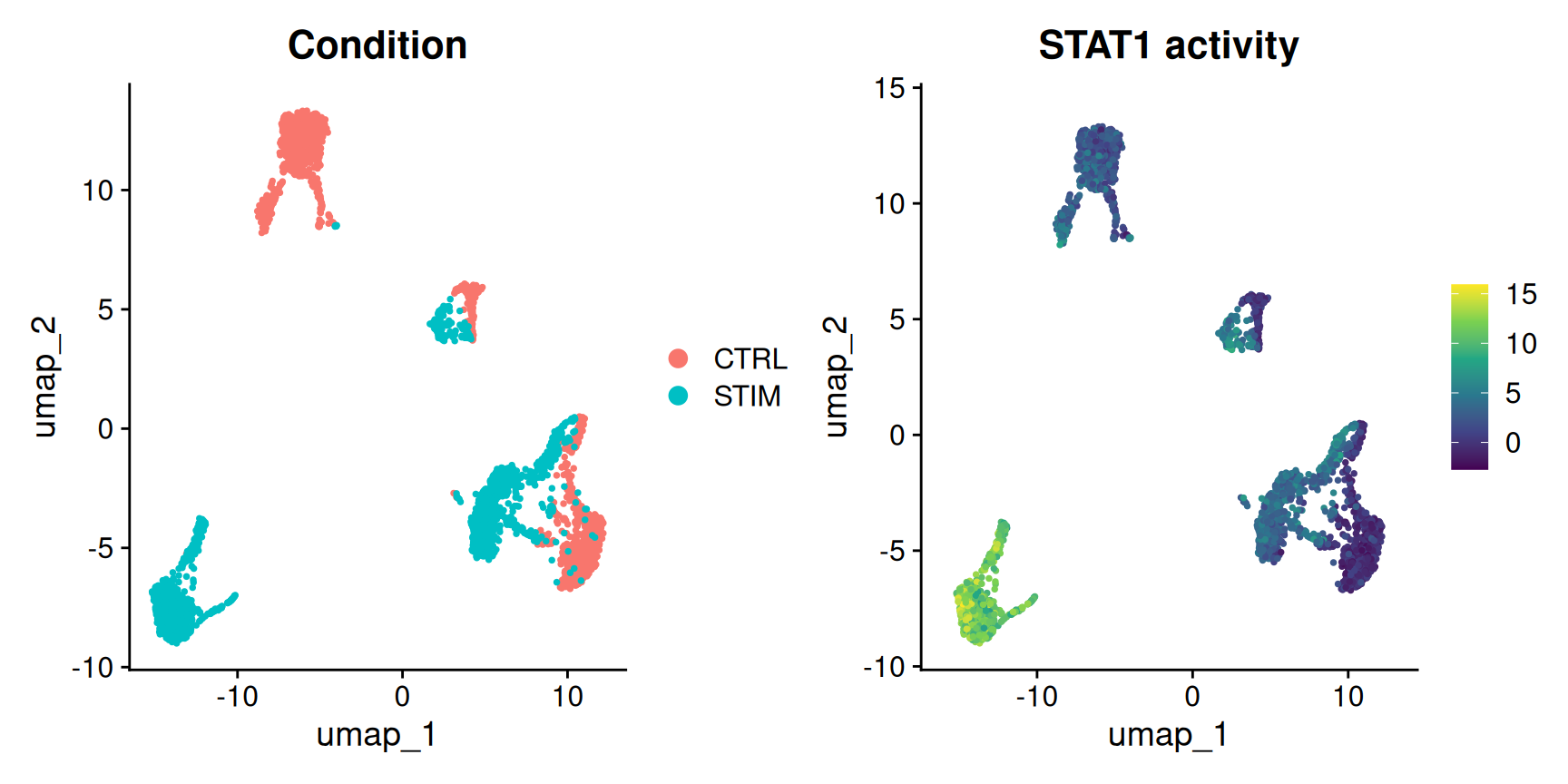
TF activity is a per-cell quantity, so it drops straight onto a UMAP (uniform manifold approximation and projection — the 2-D embedding of the cells). Colouring the map by STAT1 activity shows the interferon response as a region of the tissue lighting up, tracking the stimulated cells wherever they sit.

set.seed(42)
library(Seurat)
library(decoupleR)
library(dorothea)
library(patchwork)
library(ggplot2)

d <- readRDS("_data/ifnb_subset.rds")
obj <- CreateSeuratObject(counts = d$counts, meta.data = d$meta)
obj <- NormalizeData(obj, verbose = FALSE)
mat <- as.matrix(GetAssayData(obj, layer = "data"))
data("dorothea_hs", package = "dorothea")
net <- dorothea_hs[dorothea_hs$confidence %in% c("A", "B", "C"), ]

acts <- run_ulm(mat, net, .source = "tf", .target = "target", .mor = "mor", minsize = 5)
acts <- acts[acts$statistic == "ulm", ]
s1 <- acts[acts$source == "STAT1", ]
obj$STAT1 <- s1$score[match(colnames(obj), s1$condition)]

# Standard embedding so the score has a map to land on
obj <- FindVariableFeatures(obj, nfeatures = 2000, verbose = FALSE) |>
  ScaleData(verbose = FALSE) |> RunPCA(npcs = 30, verbose = FALSE) |>
  RunUMAP(dims = 1:30, verbose = FALSE)

p1 <- DimPlot(obj, group.by = "stim") + ggtitle("Condition")
p2 <- FeaturePlot(obj, features = "STAT1") +
  scale_color_viridis_c() + ggtitle("STAT1 activity")
p1 + p2

The two panels are almost the same picture: the region the UMAP fills with stimulated cells is exactly the region the STAT1 map paints bright. A transcription-factor activity you inferred from downstream targets reproducing the experimental condition you can see in the embedding — that is the visual form of the validation.

Where each transcription factor is active across cell types

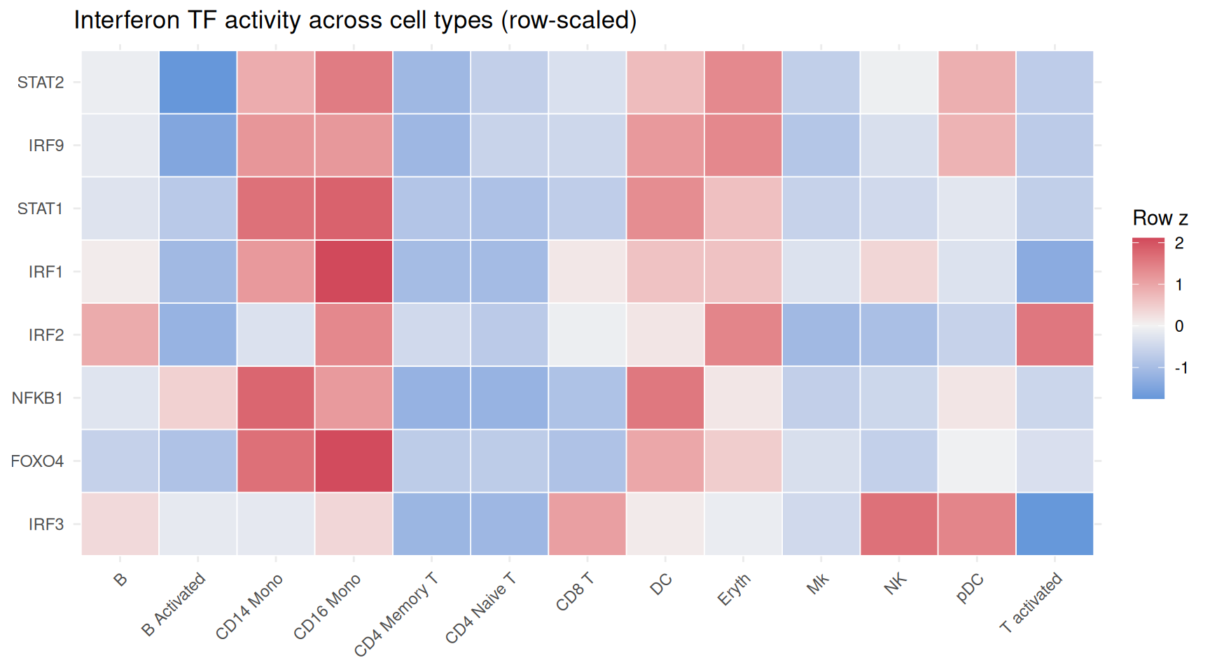
The barplot collapsed each TF to one number per condition. Activity also varies across cell types, and a heatmap of the top interferon TFs over the 13 annotated cell types shows the landscape. To compare cell-type patterns on a common scale, we scale each TF (row) to a z-score across cell types — so each row shows where, relatively, that transcription factor is most active.

library(Seurat)
library(decoupleR)
library(dorothea)
library(ggplot2)

d <- readRDS("_data/ifnb_subset.rds")
obj <- CreateSeuratObject(counts = d$counts, meta.data = d$meta)
obj <- NormalizeData(obj, verbose = FALSE)
mat <- as.matrix(GetAssayData(obj, layer = "data"))
data("dorothea_hs", package = "dorothea")
net <- dorothea_hs[dorothea_hs$confidence %in% c("A", "B", "C"), ]

acts <- run_ulm(mat, net, .source = "tf", .target = "target", .mor = "mor", minsize = 5)
acts <- acts[acts$statistic == "ulm", ]
acts$ct <- obj$seurat_annotations[match(acts$condition, colnames(obj))]

# The interferon transcription factors, mean activity per TF per cell type, row z-scored
tfs <- c("STAT2", "IRF9", "STAT1", "IRF1", "IRF2", "NFKB1", "FOXO4", "IRF3")
sub <- acts[acts$source %in% tfs, ]
mn  <- tapply(sub$score, list(sub$source, sub$ct), mean)
z   <- t(scale(t(mn)))    # row-wise z-score across cell types

df <- data.frame(tf        = rownames(z)[row(z)],
                 cell_type = colnames(z)[col(z)],
                 z         = as.vector(z))
df$tf <- factor(df$tf, levels = rev(tfs))
ggplot(df, aes(cell_type, tf, fill = z)) +
  geom_tile(color = "white", linewidth = 0.3) +
  scale_fill_gradient2(low = "#3a86d4", mid = "grey95", high = "#d1495b",
                       midpoint = 0, name = "Row z") +
  labs(x = NULL, y = NULL, title = "Interferon TF activity across cell types (row-scaled)") +
  theme_minimal(base_size = 11) +
  theme(axis.text.x = element_text(angle = 45, hjust = 1))

The interferon signal is not spread evenly. The interferon transcription factors peak in the myeloid compartment — CD14 and CD16 monocytes and dendritic cells — the professional responders that mount the strongest interferon program. A single condition-level number would have hidden that; the per-cell scores let you see which cells each transcription factor is most active in.

Methods, honesty and reproducibility

A few things to keep straight so you use these tools accurately and reproducibly.

run_ulm is one of several decoupleR methods. For TF activity the univariate linear model is the documented default: it scores each transcription factor on its own regulon, which is the right model when regulons overlap little. decoupleR also offers run_mlm (a multivariate model that fits all sources jointly, the default for a dense resource like PROGENy), run_wsum / run_wmean (weighted sums/means), and decouple() / run_consensus to combine several methods. For DoRothEA/CollecTRI TF activity, run_ulm is the sensible default.

A TF’s activity is not its own expression — that is the whole point. Do not sanity-check a TF activity score against the TF’s own transcript. STAT1’s mRNA is nearly flat between conditions while its inferred activity jumps sevenfold, because activity is read from the regulon’s targets, not from STAT1 itself. If you plot a TF’s own gene and see little change, that is expected, not a bug.

DoRothEA here, CollecTRI for live work. As noted above, dorothea::dorothea_hs is offline and deterministic, whereas decoupleR::get_collectri() fetches the newer resource from the OmnipathR web service (network-dependent, non-reproducible). The results on this page were produced with the packaged DoRothEA and are byte-stable across renders; for new analyses, CollecTRI is the more comprehensive and recommended resource.

The R decoupleR package is now the legacy interface. As of 2025 the Saez-Rodriguez lab has unified development on the Python decoupler 2.0, a faster, more memory-efficient reimplementation that is part of the scverse single-cell ecosystem; the R package is described as the legacy version and is in maintenance. The R package still works and is taught here because it plugs straight into a Seurat-based R workflow — but if you are building new pipelines, especially in Python/scanpy, that is the direction of travel. The concepts — regulons, footprint inference, ULM/MLM — are identical across both.

When to use TF activity vs pathway activity vs signature scoring

The three functional-inference methods answer different questions; choose by what you want to name.

• Reach for DoRothEA/CollecTRI + decoupleR when the question is which transcription factor — the specific regulators driving a program, from hundreds of TFs, read from their regulons. This is the finest-grained of the three: it names STAT1 and IRF9, not just “the interferon pathway”.
• Reach for pathway activity (PROGENy + decoupleR) when the question is which signaling pathway — a broad, ~14-pathway summary of the signaling systems that are on. Coarser than TF activity, but a compact overview.
• Reach for signature scoring (AUCell, UCell) when you have a curated gene set — a lineage, a cell state, a custom module — whose membership you want to quantify per cell.

In practice they layer: score your curated signatures, read the pathway footprints for the signaling systems, and infer TF activity to name the regulators behind the response. All three validate the same way — against a known contrast, as we did here with the IFN-β ground truth.

Common issues

get_collectri() or get_dorothea() hangs or errors about OmnipathR / a network connection. These convenience functions download the regulons from the OmnipathR web service, which needs internet and can stall behind a firewall — and its remote resource can change, so results are not reproducible. For a reproducible lesson use the offline packaged regulons instead: data("dorothea_hs", package = "dorothea"), then filter to confidence %in% c("A","B","C"). It is offline, deterministic, and identical in structure to what decoupleR expects. (For live work where reproducibility is handled separately, CollecTRI is the more comprehensive resource.)

A transcription factor’s own gene looks flat but its inferred activity is high. That is not a bug — it is the reason to infer activity at all. A TF is frequently regulated by phosphorylation or nuclear translocation, not transcription, so its mRNA barely moves while it switches on hundreds of targets. The activity score reads those targets (the regulon), so it can be high even when the TF’s own transcript is unchanged. Never validate a TF score against the TF’s own expression.

A transcription factor is dropped, or its score is built on very few genes. The minsize = 5 argument drops any TF whose regulon has fewer than five targets present in your matrix. If TFs you expect are missing, check that your feature names match the regulons’ gene symbols (symbols vs Ensembl IDs, species capitalization) — a naming mismatch silently starves the regulon. Including confidence tier C (as we do) already broadens coverage; lower minsize only if you accept that a score on very few targets is noisy.

Frequently asked questions

NoteWhat is the difference between transcription-factor activity and pathway activity?

Both are footprint models — they infer a regulator’s activity from the genes it affects, not from its own expression — but at different resolutions. Pathway activity with PROGENy summarises the transcriptome into about 14 broad signaling pathways (JAK-STAT, NF-κB, …). TF activity with DoRothEA/CollecTRI goes finer: it names the individual transcription factors — STAT1, STAT2, IRF9 — from hundreds of regulators. Pathways tell you the system that is signaling; TFs tell you the specific switches being thrown.

NoteDoRothEA vs CollecTRI — which regulon resource should I use?

For new analyses, CollecTRI — it is the newer, more comprehensive successor, covering many more transcription factors (Müller-Dott et al., 2023), fetched with decoupleR::get_collectri(). DoRothEA (Garcia-Alonso et al., 2019) is the older resource with confidence tiers A–E; it is used in this lesson because it ships as offline package data, which keeps the rendered numbers reproducible. get_collectri() fetches over the network (OmnipathR), so it is not reproducible in a frozen document — but in live work, prefer CollecTRI.

NoteWhy not just look at the transcription factor’s own expression?

Because a TF’s mRNA is a poor readout of its activity. Transcription factors are commonly switched on by phosphorylation or nuclear translocation, not by transcription, so the TF’s own gene can stay flat while it drives hundreds of targets. Reading the regulon — the coordinated expression of the target genes the TF controls — recovers the activity the TF’s own transcript hides. In this lesson STAT1’s activity jumps sevenfold between conditions while its own mRNA barely moves.

NoteWhat are the DoRothEA confidence levels A–E, and which should I keep?

Each DoRothEA regulon edge is graded from A (highest confidence — curated, multiple lines of evidence) to E (lowest — predicted only), reflecting how well-supported the TF-to-target link is. The standard practice is to keep the high-confidence tiers A, B and C and drop D/E, which trades a little coverage for much cleaner regulons. That is the confidence %in% c("A","B","C") filter used here — it gives 13,223 edges across 271 transcription factors.

Noterun_ulm vs run_mlm — which decoupleR method should I use for TF activity?

run_ulm (univariate linear model) scores each transcription factor on its own regulon, one at a time, and is the documented default for TF activity with DoRothEA/CollecTRI. run_mlm (multivariate) fits all sources jointly, so a source’s score is adjusted for targets it shares with others — the sensible default for a dense resource like PROGENy, but less suited to a large sparse regulon network. decoupleR also offers run_wsum, run_wmean and a consensus over methods.

Test your understanding

ImportantYour turn: which cell type has the highest STAT2 activity?

Using ifnb_subset.rds and the DoRothEA A/B/C regulons, infer TF activity with run_ulm, then find which annotated cell type has the highest mean STAT2 activity in the stimulated cells only. Does the interferon response concentrate where you would expect — the myeloid compartment?

TipHint

After run_ulm, filter the output to statistic == "ulm" and source == "STAT2". Map each cell’s condition (the barcode) to obj$stim and obj$seurat_annotations, keep only the STIM cells, then tapply(score, cell_type, mean) and sort descending.

TipSolution

library(Seurat); library(decoupleR); library(dorothea)
d <- readRDS("_data/ifnb_subset.rds")
obj <- CreateSeuratObject(counts = d$counts, meta.data = d$meta)
obj <- NormalizeData(obj, verbose = FALSE)
mat <- as.matrix(GetAssayData(obj, layer = "data"))
data("dorothea_hs", package = "dorothea")
net <- dorothea_hs[dorothea_hs$confidence %in% c("A", "B", "C"), ]

set.seed(42)
acts <- run_ulm(mat, net, .source = "tf", .target = "target", .mor = "mor", minsize = 5)
acts <- acts[acts$statistic == "ulm", ]

s2 <- acts[acts$source == "STAT2", ]
s2$stim <- obj$stim[match(s2$condition, colnames(obj))]
s2$ct   <- obj$seurat_annotations[match(s2$condition, colnames(obj))]

# STAT2 activity by cell type, stimulated cells only
sort(tapply(s2$score[s2$stim == "STIM"], s2$ct[s2$stim == "STIM"], mean), decreasing = TRUE)

STAT2 activity in the stimulated cells is highest in the myeloid cell types — the CD14 and CD16 monocytes and dendritic cells — the professional interferon responders, with the lymphoid subsets lower. That is exactly where a type-I interferon program should peak, and it is a second, cell-type-level confirmation (beyond the condition contrast) that the inferred TF activity is tracking real biology.

NoteQuick check: STAT1’s own mRNA barely differs between the control and stimulated cells, yet its inferred activity is far higher in the stimulated cells. How can that be?

A. The activity score must be wrong — a TF’s activity should track its own expression. B. TF activity is inferred from the TF’s regulon — the coordinated expression of the target genes it regulates — not from the TF’s own transcript; interferon activates STAT1 post-transcriptionally, so its targets rise (and its activity with them) even though STAT1’s own mRNA is nearly flat. C. The score is high only because the data was not normalized.

TipShow answer

B. That is exactly what regulon-based inference is designed to catch. Transcription factors are frequently switched on by phosphorylation or nuclear translocation rather than by transcription, so the TF’s own mRNA is a poor readout of its activity. run_ulm reads STAT1’s activity from its regulon — the target genes that respond when STAT1 is active — which rise sharply under IFN-β, so the inferred activity jumps even though STAT1’s own transcript barely moves. (Answer A has the logic backwards; C is wrong — the pipeline normalizes with NormalizeData and the contrast is real.)

Conclusion

Signature scoring asks whether a cell expresses a gene set; pathway activity asks whether a signaling pathway is firing; transcription-factor activity asks which regulator is driving the program — inferred from the TF’s regulon, the target genes it controls, not from the TF’s own transcript. DoRothEA supplies the regulons and decoupleR’s run_ulm scores them in every cell. On the IFN-β benchmark the method recovered the ground truth cleanly: the transcription factors that jumped most were STAT2, IRF9, STAT1 and IRF1 — the ISGF3 complex and the IRF family, the canonical type-I interferon TFs — with activity read from target genes alone while the TFs’ own transcripts stayed flat, and the myeloid cells driving the response. Keep the high-confidence regulons (tiers A/B/C), validate against a known contrast, prefer CollecTRI for live work and DoRothEA for reproducible output. TF activity completes the functional-inference trilogy alongside pathway activity and signature scoring — three complementary levels, from a curated gene set to the individual regulators cells switch on.

Related lessons

• Per-cell pathway activity with decoupleR & PROGENy — the direct companion: the same decoupleR engine on signaling-pathway footprints instead of TF regulons, validated against the same interferon contrast. · Per-cell gene signature scoring with AUCell & UCell — the membership-based first level of the trilogy. · Marker genes & cell-type annotation — supplies the cell-type labels the heatmap groups by. · Clustering & UMAP — builds the embedding the TF scores are painted on. · Bioinformatics — the pillar.
• Where this fits: signature scoring → pathway activity → transcription-factor activity with DoRothEA & decoupleR — three levels of functional inference, from a curated gene set to signaling pathways to the individual transcription factors driving the response.

🟢 With an AI agent

Ask Prova “how do I infer per-cell transcription-factor activity on my own Seurat object with DoRothEA regulons and decoupleR, and validate it against a known contrast?” — it answers with R code you can run on your own data: load the regulons, filter to high-confidence tiers, call run_ulm(), add the scores to your object, and check them against a condition you already know. The runtime is the judge. Ask Prova →

Was this page helpful?

Prove you can do it. Master the whole Single-Cell RNA-Seq Analysis in R series — track your path, build projects, and earn a certificate.

Start free →

Go Pro — unlimited Prova on your own data and a verifiable certificate that proves the skill.

from $15/mo billed yearly

Go Pro →

✓ You're Pro — keep going. The runtime is the judge.

Get new R & Python lessons by email

Practical, reproducible, no spam. Unsubscribe anytime.

Double opt-in. We never share your email.

Share this pageXLinkedInRedditHN

Note

This lesson is reproducible: every figure and number was produced by the code shown, rendered offline in the datanovia/quarto-bioinformatics Docker image — copy any block and run it to reproduce them. The runtime is the judge.

References

• Garcia-Alonso, L., Holland, C. H., Ibrahim, M. M., Türei, D., & Saez-Rodriguez, J. (2019). Benchmark and integration of resources for the estimation of human transcription factor activities — introduces the DoRothEA regulons. Genome Research, 29(8), 1363–1375. https://doi.org/10.1101/gr.240663.118
• Müller-Dott, S., Tsirvouli, E., Vazquez, M., Ramirez Flores, R. O., Badia-i-Mompel, P., Fallegger, R., Türei, D., Lægreid, A., & Saez-Rodriguez, J. (2023). Expanding the coverage of regulons from high-confidence prior knowledge for accurate estimation of transcription factor activities — introduces CollecTRI. Nucleic Acids Research, 51(20), 10934–10949. https://doi.org/10.1093/nar/gkad841
• Badia-i-Mompel, P., Vélez Santiago, J., Braunger, J., Geiss, C., Dimitrov, D., Müller-Dott, S., Taus, P., Dugourd, A., Holland, C. H., Ramirez Flores, R. O., & Saez-Rodriguez, J. (2022). decoupleR: ensemble of computational methods to infer biological activities from omics data. Bioinformatics Advances, 2(1), vbac016. https://doi.org/10.1093/bioadv/vbac016
• Kang, H. M., et al. (2018). Multiplexed droplet single-cell RNA-sequencing using natural genetic variation — the source of the IFN-β–stimulated PBMC dataset. Nature Biotechnology, 36, 89–94. https://doi.org/10.1038/nbt.4042