Per-Cell Gene Signature Scoring in R with AUCell & UCell

Quantify how strongly each cell expresses a gene program — an interferon module, a lineage signature, a pathway — with AUCell and UCell, then validate the score against a known biological contrast

A practical guide to per-cell gene-signature scoring for single-cell RNA-seq in R. Score an interferon-response module, a T-cell signature and a monocyte signature per cell with the rank-based standards AUCell and UCell, compare them against GSVA, ssGSEA and singscore, and validate every score against the built-in interferon-beta ground truth in the immune-PBMC benchmark.

TipKey takeaways

• Signature scoring turns a gene set into one number per cell. Once you have clusters and cell-type labels, the next question is often how strongly does each cell express this program? — an interferon response, a lineage identity, a pathway. A signature score answers it per cell, on a continuum, without drawing new cluster boundaries.
• AUCell and UCell are the modern single-cell standards, and both are rank-based. They score each cell from the ranking of the signature’s genes within that cell, so they are robust to sequencing depth and to the sparsity of single-cell data — no cross-cell normalization of the score needed (Aibar et al., 2017; Andreatta & Carmona, 2021).
• UCell is one call on a Seurat object; AUCell is build-rankings then score. AddModuleScore_UCell(obj, features = sigs) adds a score column per signature; AUCell splits into AUCell_buildRankings() then AUCell_calcAUC(). Large reference atlases score gene programs this way — the BoneMarrowMap human-bone-marrow atlas scores its stem-cell signatures per cell with AUCell (Zeng et al., 2025).
• GSVA, ssGSEA and singscore are the alternatives — designed for bulk, usable on single cells. GSVA and ssGSEA give a signed, bidirectional enrichment; singscore is a single-sample rank score. They agree with AUCell/UCell on strong signals, but for sparse single-cell data the rank-based per-cell methods are the default.
• Always validate a signature against a known contrast before you trust it. Here the data has a built-in ground truth — half the cells were stimulated with interferon-beta — so an interferon-gene signature must score higher in the stimulated cells. Every method recovers that. Sanity-checking against a known biology is the discipline that separates a real signal from a plausible-looking artifact.

Introduction

You have run the standard single-cell RNA-seq (scRNA-seq) workflow: quality control, normalization, clustering, and cell-type annotation. You have a map of what cells are there. But a great deal of biology is not a cell type at all — it is a program that cells switch on to different degrees: an interferon response, a cell-cycle state, an exhaustion signature, a metabolic pathway. Those live on a continuum, and a discrete cluster label throws that continuum away.

This lesson answers a different question than annotation does. Not “what type is this cell?” but “how strongly does this cell express this particular gene program?” The tool is gene-signature scoring: you hand the method a curated set of genes — a signature — and it returns a single number per cell measuring how enriched that cell is for the set. The two rank-based methods that lead in single cell are AUCell and UCell; the established alternatives are GSVA, ssGSEA and singscore.

We work on the classic IFN-β immune-PBMC benchmark: peripheral blood mononuclear cells (PBMCs — the immune cells in blood) split into a control group and a group stimulated with interferon-beta (IFN-β), a cytokine that drives a strong, well-characterized transcriptional response (Kang et al., 2018). That design gives us a built-in ground truth: a signature of interferon-stimulated genes (ISGs — genes switched on by interferon signaling) must score higher in the stimulated cells than the controls. If a scoring method cannot recover a contrast that strong, we should not trust it on a subtle one.

What per-cell signature scoring is — and when to use it

A signature is just a set of genes that mark a program: ISG15, IFIT1, MX1 and friends for an interferon response; CD3D, CD3E, IL7R for T cells. A signature score collapses that set into one number per cell — high when the cell strongly expresses the set, low when it does not. You are moving from a matrix of ~13,000 genes to a handful of interpretable per-cell scores, one per program you care about.

Use signature scoring when you want to:

• Quantify a known program per cell — an interferon response, a hypoxia signature, a stemness or exhaustion program — and see how it varies within and across your clusters, rather than only between them.
• Score a cell state that spans several cell types — cell cycle, stress, or a treatment response is not a single cluster; a score captures it wherever it appears.
• Compare a curated gene set across conditions or samples on a common, per-cell scale.

Do not reach for it when a single marker gene already answers the question, or when the “signature” is one or two genes — a score over a two-gene set is just a noisy average, and you may as well plot the genes. The method earns its keep when the program is distributed across many genes and you want the collective signal.

The data: interferon-stimulated PBMCs with a built-in ground truth

The committed ifnb_subset.rds is a balanced slice of the Kang IFN-β benchmark: a raw count matrix of 13,565 genes across 3,000 cells, plus a metadata table. The stim column records whether each cell was a CTRL (control) or STIM (IFN-β–stimulated) cell — 1,500 of each — and seurat_annotations holds the 13 cell types already called for us. We never use those labels to build the score; we hold them back to validate it.

library(Seurat)

d <- readRDS("_data/ifnb_subset.rds")
obj <- CreateSeuratObject(counts = d$counts, meta.data = d$meta)
obj <- NormalizeData(obj, verbose = FALSE)

dim(obj)                       # genes x cells

[1] 13565  3000

table(obj$stim)                # the control / IFN-beta contrast: our ground truth

CTRL STIM 
1500 1500 

table(obj$seurat_annotations)  # 13 annotated cell types

   CD14 Mono  CD4 Naive T CD4 Memory T    CD16 Mono            B        CD8 T 
         925          534          370          255          194          182 
 T activated           NK           DC  B Activated           Mk          pDC 
         125          144          106           77           52           23 
       Eryth 
          13 

Log-normalization (NormalizeData) is the one preprocessing step every method here assumes: the score is computed on the normalized expression, not raw counts. Every block below rebuilds from exactly this point, so you can copy any one of them and run it on its own.

Define the signatures

We score three signatures. The first is the star of the validation: eight canonical interferon-stimulated genes, the core of the IFN-β response. The other two are lineage signatures — a T-cell set and a monocyte set — that should light up in their own cell types, a second, orthogonal check that the scores are meaningful.

sigs <- list(
  ISG      = c("ISG15", "IFI6", "IFIT1", "IFIT3", "MX1", "OAS1", "ISG20", "IRF7"),  # interferon-stimulated
  Tcell    = c("CD3D", "CD3E", "CD8A", "IL7R", "CCR7"),                             # T-cell identity
  Monocyte = c("CD14", "LYZ", "S100A8", "S100A9", "FCN1"))                          # monocyte identity

lengths(sigs)   # genes per signature

     ISG    Tcell Monocyte 
       8        5        5 

A practical signature is usually 20–200 genes; ours are deliberately small and hand-picked so the biology is transparent. The rank-based methods below are robust to signature size, but a set of only a handful of genes gives the score less to work with — prefer a curated set of tens of genes in real work.

AUCell: rank each cell, score the area under the curve

AUCell (area under the curve, per cell) was introduced with SCENIC to score regulon activity in single cells (Aibar et al., 2017). The idea is elegant and depth-robust: within each cell, rank all genes by expression; then ask how near the top of that ranking the signature genes sit. Concretely it computes, per cell, the area under the recovery curve (the AUC) of the signature genes across the ranking — high when the signature’s genes are among the cell’s most-expressed genes, low when they are scattered down the list. Because it uses only the ranking within each cell, it does not care about absolute counts or sequencing depth.

It runs in two steps. AUCell_buildRankings() ranks the genes within every cell once; AUCell_calcAUC() then scores any number of signatures against those rankings.

library(Seurat)
library(AUCell)
library(ggplot2)

d <- readRDS("_data/ifnb_subset.rds")
obj <- CreateSeuratObject(counts = d$counts, meta.data = d$meta)
obj <- NormalizeData(obj, verbose = FALSE)
sigs <- list(
  ISG      = c("ISG15", "IFI6", "IFIT1", "IFIT3", "MX1", "OAS1", "ISG20", "IRF7"),
  Tcell    = c("CD3D", "CD3E", "CD8A", "IL7R", "CCR7"),
  Monocyte = c("CD14", "LYZ", "S100A8", "S100A9", "FCN1"))

set.seed(42)
rankings <- AUCell_buildRankings(GetAssayData(obj, layer = "data"),
                                 plotStats = FALSE, verbose = FALSE)
auc  <- AUCell_calcAUC(sigs, rankings, verbose = FALSE)
aucm <- getAUC(auc)                       # signatures x cells (3 x 3000)

# The money result: the ISG score MUST be higher in the stimulated cells
tapply(aucm["ISG", ], obj$stim, mean)

      CTRL       STIM 
0.08742204 0.75932580 

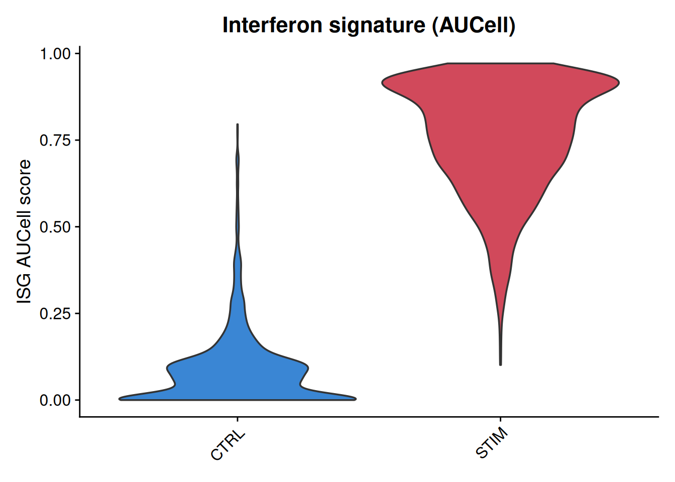
obj$ISG_AUCell <- aucm["ISG", ]
VlnPlot(obj, features = "ISG_AUCell", group.by = "stim", pt.size = 0,
        cols = c(CTRL = "#3a86d4", STIM = "#d1495b")) +
  labs(title = "Interferon signature (AUCell)", x = NULL, y = "ISG AUCell score") +
  theme(legend.position = "none")

The mean ISG AUCell score is 0.087 in the controls and 0.759 in the stimulated cells — an eight-to-nine-fold separation, and the violins barely overlap. AUCell recovered the experimental condition from an eight-gene signature alone, without ever being told which cells were stimulated. That is exactly the validation you want to see before trusting a score on a question you don’t already know the answer to. Large reference atlases lean on this: the BoneMarrowMap atlas scores its hematopoietic-stem-cell signatures per cell with AUCell (score_Genesets_AUCell) to place query cells on a differentiation map (Zeng et al., 2025).

UCell: the same idea, one call on the Seurat object

UCell takes the same rank-based philosophy and packages it for the Seurat workflow (Andreatta & Carmona, 2021). Its score is based on the Mann-Whitney U statistic: for each cell it asks whether the signature genes rank significantly higher than the rest, normalized to a 0–1 scale. It is deterministic, memory-frugal, robust to dataset size, and — the practical win — it works directly on the Seurat object and adds the scores straight to the metadata.

library(Seurat)
library(UCell)

d <- readRDS("_data/ifnb_subset.rds")
obj <- CreateSeuratObject(counts = d$counts, meta.data = d$meta)
obj <- NormalizeData(obj, verbose = FALSE)
sigs <- list(
  ISG      = c("ISG15", "IFI6", "IFIT1", "IFIT3", "MX1", "OAS1", "ISG20", "IRF7"),
  Tcell    = c("CD3D", "CD3E", "CD8A", "IL7R", "CCR7"),
  Monocyte = c("CD14", "LYZ", "S100A8", "S100A9", "FCN1"))

# One call: scores every signature, adds ISG_UCell / Tcell_UCell / Monocyte_UCell columns
obj <- AddModuleScore_UCell(obj, features = sigs, name = "_UCell")

tapply(obj$ISG_UCell, obj$stim, mean)   # same contrast, UCell scale

     CTRL      STIM 
0.1361304 0.8341464 

UCell tells the same story on its own scale: the ISG score averages 0.136 in the controls and 0.834 in the stimulated cells. The absolute numbers differ from AUCell’s (each method has its own scale), but the conclusion is identical and just as clean — the interferon program is on in the stimulated cells and off in the controls. Two independent rank-based methods agreeing is itself reassurance.

See the score on the map

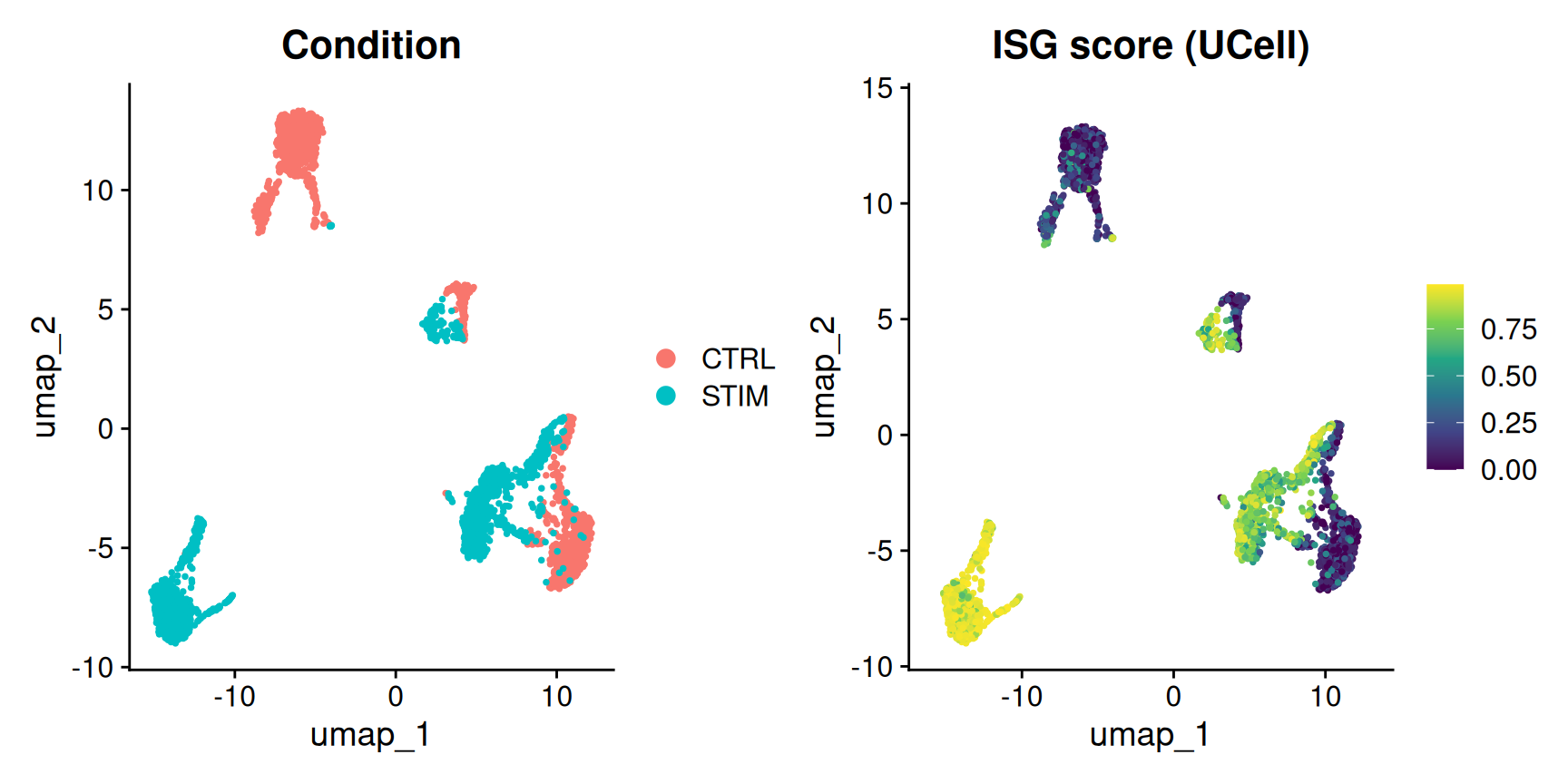
A signature score is a per-cell quantity, so it drops straight onto a UMAP (uniform manifold approximation and projection — the 2-D embedding of the cells). Colouring the map by the ISG UCell score shows the interferon response as a gradient across the tissue: whole regions light up, tracking the stimulated cells wherever they sit.

set.seed(42)
library(Seurat)
library(UCell)
library(patchwork)

d <- readRDS("_data/ifnb_subset.rds")
obj <- CreateSeuratObject(counts = d$counts, meta.data = d$meta)
sigs <- list(ISG = c("ISG15", "IFI6", "IFIT1", "IFIT3", "MX1", "OAS1", "ISG20", "IRF7"))

obj <- NormalizeData(obj, verbose = FALSE) |>
  FindVariableFeatures(nfeatures = 2000, verbose = FALSE) |> ScaleData(verbose = FALSE) |>
  RunPCA(npcs = 30, verbose = FALSE) |> RunUMAP(dims = 1:30, verbose = FALSE)
obj <- AddModuleScore_UCell(obj, features = sigs, name = "_UCell")

p1 <- DimPlot(obj, group.by = "stim") + ggtitle("Condition")
p2 <- FeaturePlot(obj, features = "ISG_UCell") +
  scale_color_viridis_c() + ggtitle("ISG score (UCell)")
p1 + p2

The two panels are almost the same picture: the region the UMAP fills with stimulated cells is exactly the region the ISG score paints bright. That correspondence — a score you computed from eight genes reproducing the experimental condition you can see in the embedding — is the visual form of the validation.

The lineage signatures land on the right cells

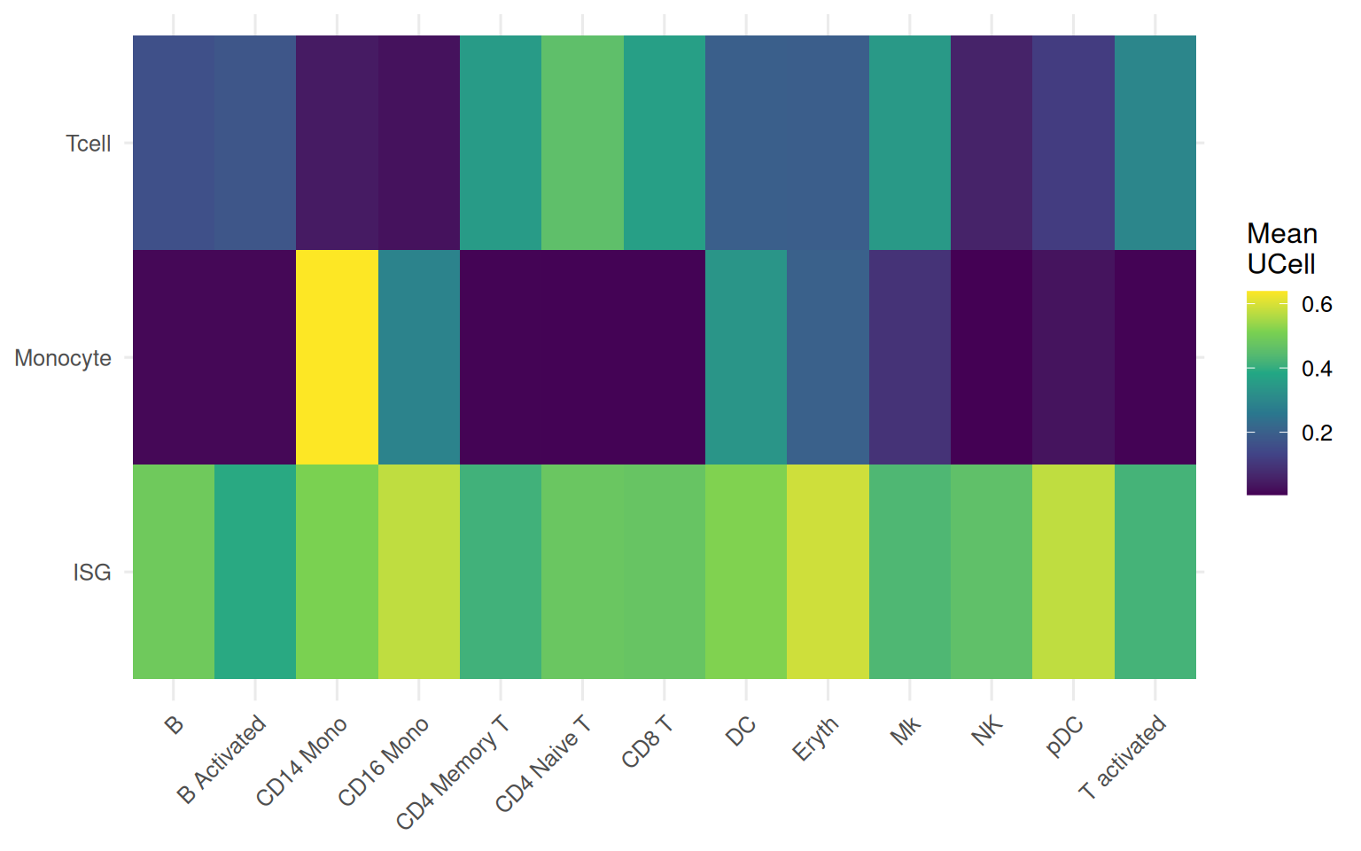
The interferon signature is condition-driven; the T-cell and monocyte signatures are identity-driven, so they give a second, orthogonal check. Average each UCell score within each annotated cell type and lay it out as a heatmap: a good signature should peak in exactly the cell type it marks.

library(Seurat)
library(UCell)
library(ggplot2)

d <- readRDS("_data/ifnb_subset.rds")
obj <- CreateSeuratObject(counts = d$counts, meta.data = d$meta)
obj <- NormalizeData(obj, verbose = FALSE)
sigs <- list(
  ISG      = c("ISG15", "IFI6", "IFIT1", "IFIT3", "MX1", "OAS1", "ISG20", "IRF7"),
  Tcell    = c("CD3D", "CD3E", "CD8A", "IL7R", "CCR7"),
  Monocyte = c("CD14", "LYZ", "S100A8", "S100A9", "FCN1"))
obj <- AddModuleScore_UCell(obj, features = sigs, name = "_UCell")

# Mean score per signature per cell type (base R aggregation)
cols <- c("ISG_UCell", "Tcell_UCell", "Monocyte_UCell")
m <- sapply(cols, function(col) tapply(obj[[col]][, 1], obj$seurat_annotations, mean))
colnames(m) <- c("ISG", "Tcell", "Monocyte")

# Where does each lineage signature peak?
sort(m[, "Tcell"],    decreasing = TRUE)[1:3]

 CD4 Naive T        CD8 T CD4 Memory T 
   0.4571680    0.3630815    0.3510867 

sort(m[, "Monocyte"], decreasing = TRUE)[1:3]

CD14 Mono        DC CD16 Mono 
0.6385011 0.3369248 0.2883582 

df <- data.frame(cell_type = rownames(m)[row(m)],
                 signature = colnames(m)[col(m)],
                 score     = as.vector(m))
ggplot(df, aes(cell_type, signature, fill = score)) +
  geom_tile() +
  scale_fill_viridis_c() +
  labs(x = NULL, y = NULL, fill = "Mean\nUCell") +
  theme_minimal(base_size = 12) +
  theme(axis.text.x = element_text(angle = 45, hjust = 1))

The lineage signatures land where they should. The T-cell score peaks in CD4 Naive T cells (0.457), followed by the other T subsets — CD8 T and CD4 Memory T. The monocyte score peaks in CD14 Mono cells (0.639), with the dendritic cells next. The interferon row is more uniformly warm, because it reflects the stimulation condition rather than a lineage — which is exactly right. Each signature reports the biology it was built for.

The chooser: GSVA, ssGSEA and singscore

AUCell and UCell are the rank-based per-cell standards, but three other methods appear constantly in the literature — usually because they came from the bulk RNA-seq world and researchers carry them over. It is worth knowing what they do and how they differ.

• GSVA (gene set variation analysis) estimates a signed enrichment score per sample by comparing each gene’s expression distribution across cells to a set-based statistic (Hänzelmann et al., 2013). Signed means the score can be negative (the program is depleted), which AUCell and UCell cannot express.
• ssGSEA (single-sample gene set enrichment analysis) is the single-sample form of GSEA: it ranks genes within a sample and integrates a running enrichment statistic over the signature (Barbie et al., 2009).
• singscore is a rank-based single-sample score, conceptually the closest of the three to UCell, and it can score a directed (up/down) or undirected signature (Foroutan et al., 2018).

A crucial API note that trips people up: GSVA 2.x uses parameter objects. The old gsva(expr, genesets) call was removed — you now build a gsvaParam() (or ssgseaParam()) object and pass that to gsva(). Here are all three scoring the ISG signature on the same data:

library(Seurat)
library(GSVA)
library(singscore)

d <- readRDS("_data/ifnb_subset.rds")
obj <- CreateSeuratObject(counts = d$counts, meta.data = d$meta)
obj <- NormalizeData(obj, verbose = FALSE)
sigs <- list(
  ISG      = c("ISG15", "IFI6", "IFIT1", "IFIT3", "MX1", "OAS1", "ISG20", "IRF7"),
  Tcell    = c("CD3D", "CD3E", "CD8A", "IL7R", "CCR7"),
  Monocyte = c("CD14", "LYZ", "S100A8", "S100A9", "FCN1"))
expr <- as.matrix(GetAssayData(obj, layer = "data"))   # dense matrix for the bulk-style methods

# GSVA 2.x: build a param object, then call gsva() on it (the old gsva(expr, sigs) API is gone)
g_gsva <- gsva(gsvaParam(expr, sigs, kcdf = "Gaussian"), verbose = FALSE)
tapply(g_gsva["ISG", ], obj$stim, mean)     # GSVA is signed: control is negative

      CTRL       STIM 
-0.8013506  0.7173729 

# ssGSEA via the same param-object interface
g_ssgsea <- gsva(ssgseaParam(expr, sigs), verbose = FALSE)
tapply(g_ssgsea["ISG", ], obj$stim, mean)

     CTRL      STIM 
0.1476112 0.8179692 

# singscore: rank the genes once, then score the ISG set
ranked <- rankGenes(expr)
ss <- simpleScore(ranked, upSet = sigs$ISG)$TotalScore
tapply(ss, obj$stim, mean)                   # singscore, ISG by condition

      CTRL       STIM 
-0.3276772  0.3873182 

All three agree with AUCell and UCell: the interferon score is far higher in the stimulated cells. GSVA goes from -0.80 (control) to +0.72 (stimulated) — the sign flip is GSVA telling you the program is depleted in controls and enriched in the stimulated cells. ssGSEA runs 0.15 → 0.82 and singscore -0.33 → 0.39. Five different methods, five different scales, one unanimous conclusion. That unanimity on a strong signal is the point: when the biology is real, the choice of scorer rarely changes the call.

Which method when

You have…	Use	Why
Single-cell data, want a robust per-cell score	UCell or AUCell	Rank-based, depth- and sparsity-robust; UCell is one call on the Seurat object, AUCell is the SCENIC-native default
Many signatures to score across a whole atlas	AUCell	Build the cell rankings once, then score any number of gene sets against them
A need for a signed score (enriched vs depleted)	GSVA	Bidirectional by design; the only method here that reports depletion
A directed up/down signature, or a bulk/pseudobulk matrix	singscore or ssGSEA	Single-sample rank scores built for bulk; handle up-and-down gene sets
Pseudobulk (aggregated per sample) rather than per cell	GSVA / ssGSEA	These were designed for the sample-level, lower-noise setting

The recommendation for single-cell work is simple: default to UCell or AUCell. They were built for the sparsity and depth variation of single cells, they need no cross-cell normalization of the score, and they scale. Reach for GSVA when you specifically need a signed enrichment, and for singscore/ssGSEA when you are working with a directed signature or a pseudobulk matrix.

Validation is the discipline, not an afterthought

The one habit that matters more than the method choice: never trust a signature score you have not validated. A scoring function will always return numbers — plausible-looking, well-distributed numbers — whether or not the signature means anything in your data. Three ways to check before you build on a score:

• Score against a known contrast. If your design has a built-in ground truth — a stimulation, a genotype, a time point — a relevant signature must move in the expected direction, as the ISG score did across CTRL and STIM here. This is the strongest check available.
• Score a positive-control signature. A lineage signature must peak in its own cell type, as the T-cell and monocyte signatures did. If a signature for a program you understand lands on the wrong cells, the scoring — or the signature — is wrong, and a subtler signature will be wrong too.
• Check gene coverage. A signature is only as good as the genes actually present in your object. If half the signature genes are missing (different naming, a filtered feature set), the score is built on the remainder — quietly weaker than you think.

Do these first, and the score becomes evidence. Skip them, and it is decoration.

Common issues

gsva(expr, sigs) errors with “unable to find an inherited method” or an argument error. You are on GSVA 2.x, where the old direct API was removed. Build a parameter object first and pass it to gsva(): gsva(gsvaParam(expr, sigs, kcdf = "Gaussian")) for GSVA, gsva(ssgseaParam(expr, sigs)) for ssGSEA. For log-normalized single-cell data use kcdf = "Gaussian"; for raw counts use kcdf = "Poisson".

Some signature genes are missing from the object, and the score looks weak. The methods silently score on whatever signature genes are present. Check the overlap before scoring — lengths(lapply(sigs, intersect, rownames(obj))) versus lengths(sigs) — and fix gene-name mismatches (symbols vs Ensembl IDs, species capitalization) so the full signature is actually used.

The scores do not separate the groups you expected. First rule out the mechanical causes: are you scoring on normalized data (NormalizeData run) rather than raw counts? Are the signature genes present (above)? Is the signature large enough — a two- or three-gene “signature” gives a noisy score? Only once those are clean does a flat score mean something biological: the program genuinely does not vary across your cells.

Frequently asked questions

NoteAUCell vs UCell vs GSVA — which should I use for single-cell data?

For single-cell RNA-seq, default to UCell or AUCell: both are rank-based, so they are robust to sequencing depth and the sparsity of single-cell data and need no cross-cell normalization of the score. UCell is a single call that adds scores to your Seurat object; AUCell builds the cell rankings once and then scores any number of signatures. GSVA and ssGSEA were designed for bulk RNA-seq and give a signed enrichment score — useful when you need to express depletion, or when you are working with pseudobulk (per-sample aggregated) data rather than individual cells.

NoteDo I need to normalize the data before scoring a signature?

Yes. Run log-normalization (NormalizeData in Seurat) first — every method here scores on normalized expression, not raw counts. The rank-based methods (AUCell, UCell, singscore) are then robust to residual depth differences because they use only the ranking of genes within each cell. For GSVA and ssGSEA on log-normalized data, set kcdf = "Gaussian"; use kcdf = "Poisson" only if you pass raw counts.

NoteHow many genes should a gene signature have?

A practical signature is usually 20–200 genes. Rank-based methods handle small sets, but a signature of only two or three genes gives a noisy score — you may as well plot the genes directly. Very large sets (many hundreds) dilute the specific signal with generically expressed genes. Curate to the genes that genuinely mark the program, and check how many are actually present in your object before trusting the score.

NoteWhat is the difference between Seurat’s AddModuleScore and UCell?

AddModuleScore (Seurat’s built-in) averages the signature genes’ expression relative to a randomly sampled control gene set — a difference-of-means score that is sensitive to sequencing depth and to the control sampling. UCell instead uses the Mann-Whitney rank statistic per cell, which is deterministic and robust to depth and dataset size. For a stable, reproducible per-cell score, UCell (or AUCell) is the more defensible choice; AddModuleScore is fine for a quick look.

NoteCan I score a signature that has both up and down genes?

Yes, but not with AUCell or UCell alone, which score a single (up) set. Use singscore with both upSet and downSet (simpleScore(ranked, upSet = up, downSet = down)) for a directed score, or GSVA, which is signed and reflects depletion as a negative score. For a purely up-regulated program — like the interferon signature here — a single-set score from UCell or AUCell is the simplest choice.

Test your understanding

ImportantYour turn: score a cell-cycle signature and validate it

Using ifnb_subset.rds, score an S-phase signature — the S-phase genes shipped with Seurat, cc.genes$s.genes — per cell with UCell, and validate it. There is no stimulation ground truth for the cell cycle here, so use a positive-control check instead: activated, proliferating subsets (the activated B and T cells, and the plasmacytoid dendritic cells) should carry a higher mean S-phase score than terminally differentiated resting cells. Compute the mean S-phase UCell score per cell type and inspect the ranking. Does the score behave like a cell-cycle score should?

TipHint

cc.genes$s.genes is a character vector of S-phase gene symbols. Pass it as a named list to AddModuleScore_UCell(obj, features = list(Sphase = cc.genes$s.genes)), then aggregate with tapply(obj$Sphase_UCell, obj$seurat_annotations, mean) and sort. Remember to intersect the signature with rownames(obj) if some genes are absent.

TipSolution

library(Seurat); library(UCell)
d <- readRDS("_data/ifnb_subset.rds")
obj <- CreateSeuratObject(counts = d$counts, meta.data = d$meta)
obj <- NormalizeData(obj, verbose = FALSE)

# S-phase signature shipped with Seurat, restricted to genes present in the object
s_sig <- intersect(cc.genes$s.genes, rownames(obj))
obj <- AddModuleScore_UCell(obj, features = list(Sphase = s_sig), name = "_UCell")

# Positive-control check: which cell types score highest for S phase?
sort(tapply(obj$Sphase_UCell, obj$seurat_annotations, mean), decreasing = TRUE)

Running the block, the proliferating and recently activated subsets — activated B cells, activated T cells, and plasmacytoid dendritic cells (pDC) — score highest, while the terminally differentiated erythrocytes sit at the bottom. That is roughly the gradient a cell-cycle score should produce: dividing and freshly activated populations above resting and post-mitotic ones. With no stimulation contrast to lean on, this positive-control ranking is your validation — a signature for a program you understand landing on the cells you expect is the evidence the score is trustworthy.

NoteQuick check: you score an interferon signature with UCell and the control and stimulated cells have nearly identical mean scores. Before concluding “no interferon response,” what should you check first?

A. Nothing — identical scores prove there is no interferon response. B. Whether the signature genes are actually present in the object and the data was log-normalized before scoring; a mismatch in gene names or scoring on raw counts can flatten a real signal. C. Re-run with a different random seed until the groups separate.

TipShow answer

B. A flat score is a result, but first rule out the mechanical causes. If the signature’s gene symbols do not match the object’s feature names (symbols vs Ensembl IDs, species capitalization), the methods silently score on the few that overlap — or none — and the score collapses. Likewise, scoring on raw counts instead of log-normalized expression distorts every method. Check gene overlap (intersect(sig, rownames(obj))) and that NormalizeData was run; only when those are clean does a flat score mean the program genuinely does not vary. (Answer C is wrong — UCell is deterministic; the seed does not change the score.)

Conclusion

Clustering tells you what cells are present; signature scoring tells you how strongly each cell runs a program. The rank-based methods UCell and AUCell are the single-cell standards — depth- and sparsity-robust, needing no cross-cell normalization, and as easy as one call on a Seurat object. On the IFN-β benchmark an eight-gene interferon signature scored ~9× higher in the stimulated cells with both, and the lineage signatures landed squarely on their own cell types — the built-in ground truth that turns a score into evidence. The bulk-world alternatives GSVA (signed), ssGSEA and singscore all agreed on the strong signal, each on its own scale, and each has its niche. But the method matters less than the habit: score against a known contrast, check a positive control, confirm your genes are present — validate first, and only then read the biology off the score. Per-cell scoring is the entry point to functional analysis; later lessons build on it to quantify pathway and transcription-factor activity across cells.

Related lessons

• Marker genes & cell-type annotation — assigns the discrete cell-type labels; signature scoring is the continuous complement, quantifying programs within and across those types. · Clustering & UMAP — builds the embedding the scores are painted on. · Integration & batch correction — the multi-sample setting where scoring a shared program across conditions is most useful. · Pseudobulk differential expression — the sample-level analysis GSVA and ssGSEA were designed for. · Bioinformatics — the pillar.
• Where this fits: clustering & UMAP → marker genes & annotation → per-cell signature scoring with AUCell & UCell → pathway- and transcription-factor-activity scoring in later lessons — from discrete cell-type labels to the continuous programs cells run.

🟢 With an AI agent

Ask Prova “how do I score a gene signature per cell on my own Seurat object with UCell and AUCell, and check that the score is trustworthy?” — it answers with R code you can run on your own data: define the signature, call AddModuleScore_UCell() (or build AUCell rankings), validate against a known contrast, and plot the score on your UMAP. The runtime is the judge. Ask Prova →

Was this page helpful?

Prove you can do it. Master the whole Single-Cell RNA-Seq Analysis in R series — track your path, build projects, and earn a certificate.

Start free →

Go Pro — unlimited Prova on your own data and a verifiable certificate that proves the skill.

from $15/mo billed yearly

Go Pro →

✓ You're Pro — keep going. The runtime is the judge.

Get new R & Python lessons by email

Practical, reproducible, no spam. Unsubscribe anytime.

Double opt-in. We never share your email.

Share this pageXLinkedInRedditHN

Note

This lesson is reproducible: every figure and number was produced by the code shown, rendered in the datanovia/quarto-bioinformatics Docker image — copy the blocks and run them in order to reproduce them. The runtime is the judge.

References

• Aibar, S., et al. (2017). SCENIC: single-cell regulatory network inference and clustering — introduces AUCell for per-cell gene-set scoring. Nature Methods, 14, 1083–1086. https://doi.org/10.1038/nmeth.4463
• Andreatta, M., & Carmona, S. J. (2021). UCell: robust and scalable single-cell gene signature scoring. Computational and Structural Biotechnology Journal, 19, 3796–3798. https://doi.org/10.1016/j.csbj.2021.06.043
• Hänzelmann, S., Castelo, R., & Guinney, J. (2013). GSVA: gene set variation analysis for microarray and RNA-seq data. BMC Bioinformatics, 14, 7. https://doi.org/10.1186/1471-2105-14-7
• Barbie, D. A., et al. (2009). Systematic RNA interference reveals that oncogenic KRAS-driven cancers require TBK1 — introduces ssGSEA. Nature, 462, 108–112. https://doi.org/10.1038/nature08460
• Foroutan, M., et al. (2018). Single sample scoring of molecular phenotypes (singscore). BMC Bioinformatics, 19, 404. https://doi.org/10.1186/s12859-018-2435-4
• Zeng, A. G. X., et al. (2025). Single-cell transcriptional atlas of human hematopoiesis (BoneMarrowMap) — scores stem-cell signatures per cell with AUCell. Blood Cancer Discovery, 6(4), 307–324. https://doi.org/10.1158/2643-3230.BCD-24-0342
• Kang, H. M., et al. (2018). Multiplexed droplet single-cell RNA-sequencing using natural genetic variation — the source of the IFN-β–stimulated PBMC dataset. Nature Biotechnology, 36, 89–94. https://doi.org/10.1038/nbt.4042