Pseudobulk Differential Expression for scRNA-Seq in R (DESeq2)
Aggregate each donor’s cells into one profile, run DESeq2 with the donors as biological replicates, and find condition-driven genes without the false positives per-cell tests produce
Bioinformatics
A practical guide to finding genes that change between conditions in multi-sample single-cell RNA-seq — the correct way. See why per-cell tests like Seurat’s FindMarkers inflate false positives on cross-condition comparisons (pseudoreplication), then aggregate each donor’s cells into a pseudobulk profile and run DESeq2 with the donors as biological replicates, on the Kang interferon-β PBMC dataset (8 donors, control vs stimulated).
Published
July 3, 2026
Modified
July 7, 2026
TipKey takeaways
Cross-condition differential expression (DE) in single-cell data has one correct method, and it is not FindMarkers. Testing every cell as an independent replicate (a per-cell Wilcoxon test) treats thousands of cells as thousands of samples — but your biological replicates are the donors, not the cells. That pseudoreplication inflates the false discovery rate (FDR): p-values become astronomically small and hundreds of genes come out “significant” even when nothing is really different.
The fix is pseudobulk. Sum each donor’s raw counts within a cell type into one profile per donor per condition, then run a standard bulk RNA-seq method — DESeq2, edgeR, or limma-voom — with the donors as replicates. This is the field’s settled best practice (Squair et al., 2021; Crowell et al., 2020).
Donors are the replicates, so a valid experiment needs several of them. We use the Kang interferon-β study — 8 donors, control vs stimulated — which is exactly why it works where the 2-sample data from the integration lesson could not: pseudobulk cannot manufacture replication you did not collect.
Block on the donor. In the DESeq2 design ~ ind + stim, ind (the donor) is a factor that soaks up donor-to-donor baseline differences so the stim effect is estimated within donor. Forgetting factor() — when the donor ID is a number — silently fits the wrong model.
The result is a clean, interpretable table: log2 fold change, an FDR-adjusted p-value, and the familiar volcano. On CD14+ monocytes the top hits are the canonical interferon-stimulated genes (ISGs) — CCL8, ISG20, IFITM2, IFIT3, ISG15 — up in the stimulated condition, exactly as the biology predicts.
Introduction
You integrated your samples, clustered them, and named the cell types. Now comes the question the experiment was built to answer: within a cell type, which genes changed with the treatment? For interferon-β–stimulated blood, which genes did the monocytes turn on in response?
The tempting shortcut is to reach for the tool you already know. Subset to the monocytes, run Seurat’s FindMarkers() comparing stimulated versus control, and you get a tidy list — often more than a thousand genes, many with p-values like 1e-80. It looks like a triumphant result. It is largely an artifact.
FindMarkers() runs a per-cell test (a Wilcoxon rank-sum test by default), and it treats every cell as an independent replicate. But two monocytes from the same donor are not independent measurements of “the monocyte response” — they share that donor’s genetics, batch, and processing. Your real biological replicates are the donors. Counting cells as replicates inflates the effective sample size from a handful of donors to thousands of cells, which crushes the p-values and inflates the FDR. This is pseudoreplication, and it is now well documented as the wrong way to do cross-condition DE in single-cell data (Squair et al., 2021; Crowell et al., 2020; Murphy & Skene, 2022).
This lesson teaches the method that fixes it: pseudobulk aggregation. You collapse each donor’s cells into a single expression profile, then hand those profiles to a bulk RNA-seq engine — here DESeq2 — with the donors as replicates and the donor as a blocking factor. We work on the Kang interferon-β PBMC dataset (peripheral blood mononuclear cells), which has eight donors measured in both conditions — the biological replication that makes the whole thing valid.
The data: eight donors, two conditions
The committed kang_subset.rds is a slice of the canonical Kang 2018 study (Kang et al., 2018): PBMCs from 8 donors, each profiled at rest (ctrl) and after interferon-β (IFN-β) stimulation (stim), across three cell types. It is stored as a raw count matrix plus a metadata table with three columns — ind (the donor), stim (the condition), and cell (the cell type).
library(Matrix)d <-readRDS("_data/kang_subset.rds")counts <- d$counts # genes x cells, raw counts (a sparse dgCMatrix)meta <- d$meta # ind (donor), stim (ctrl/stim), cell (cell type)# The design: donors x conditions x cell typestable(meta$cell, meta$stim)
                    ctrl stim
  B cells            870  888
  CD14+ Monocytes   1176 1200
  CD4 T cells       1200 1200
  CD8 T cells          0    0
  Dendritic cells      0    0
  FCGR3A+ Monocytes    0    0
  Megakaryocytes       0    0
  NK cells             0    0
length(unique(meta$ind)) # the biological replicates
[1] 8
Three cell types, each present in both conditions, and — the number that matters — 8 donors. Those donors are the biological replicates. The integration lesson used a two-sample dataset, which is enough to align samples but not enough to test a condition effect: with one donor per arm you cannot separate the treatment from that one donor’s idiosyncrasies. Cross-condition DE needs replication, and this dataset has it.
We will run the worked example on CD14+ monocytes, the strongest and clearest interferon responder.
See the problem: per-cell testing calls almost everything significant
Before fixing anything, look at what the shortcut actually does. Take the CD14+ monocytes, log-normalize exactly as Seurat does, and run one Wilcoxon test per gene comparing stimulated versus control — the same rank-sum test FindMarkers() runs by default — treating each cell as a replicate.
library(Matrix)d <-readRDS("_data/kang_subset.rds")counts <- d$counts; meta <- d$metamono <- meta$cell =="CD14+ Monocytes"cm <- counts[, mono]; mm <- meta[mono, ]# Log-normalize (what Seurat's LogNormalize does), keep genes expressed in >=10% of cellscs <- Matrix::colSums(cm)ln <-log1p(sweep(cm, 2, cs, "/") *1e4)ln <-as.matrix(ln[Matrix::rowMeans(cm >0) >=0.10, ])# One Wilcoxon rank-sum test per gene, ctrl vs stim, treating each CELL as a replicatepv <-apply(ln, 1, function(g) wilcox.test(g ~ mm$stim)$p.value)padj <-p.adjust(pv, method ="BH")c(cells_tested =ncol(ln),genes_tested =length(pv),significant =sum(padj <0.05),pct_significant =round(100*mean(padj <0.05), 1),at_p_below_1e50 =sum(pv <1e-50))
The verdict is absurd on its face: of 1,710 genes tested, 1,422 — about 83% — come out “significant” at a 5% FDR, and 254 of them sit below a raw p-value of 1e-50. No real biological comparison makes 83% of the transcriptome differentially expressed. The engine is not measuring biology; it is measuring the ~2,400 cells you fed it. With that many “replicates”, even a whisper of a difference clears any threshold. FindMarkers() gives the same picture — it runs this exact test.
Prove it is an artifact: a null with no real difference
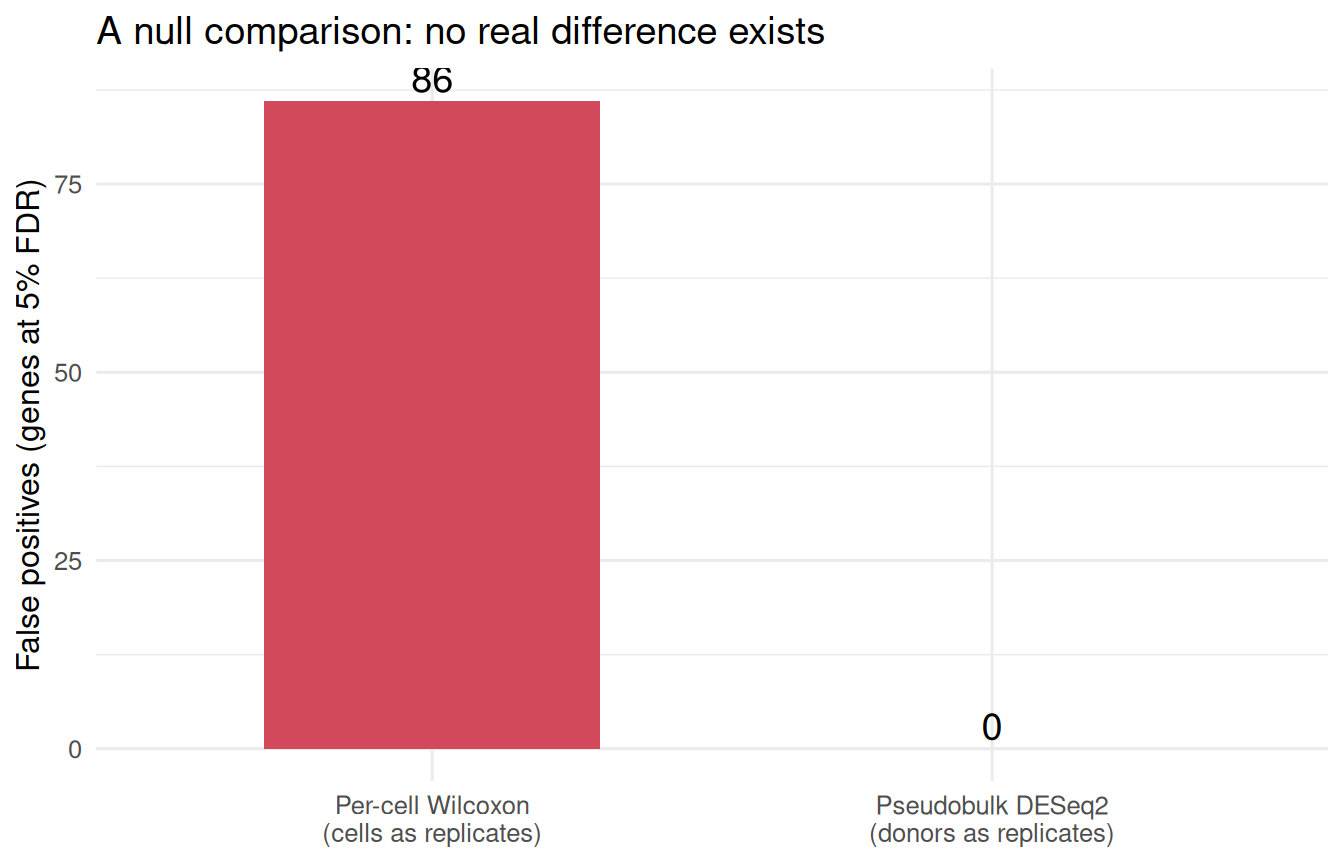
“83% is too many” is an argument. Here is the proof. Build a comparison where there is no biological difference at all — take only the control monocytes and split the 8 donors into two random groups. Any gene that comes out “significant” is, by construction, a false positive. Run both methods on this null.
library(Matrix); library(DESeq2); library(ggplot2)d <-readRDS("_data/kang_subset.rds")counts <- d$counts; meta <- d$meta# A TRUE NULL: only control monocytes, donors split into two fake groups -> no real DE existssel <- meta$cell =="CD14+ Monocytes"& meta$stim =="ctrl"cm <- counts[, sel]; mm <- meta[sel, ]set.seed(1)groupA <-sample(sort(unique(mm$ind)), 4)mm$fake <-ifelse(mm$ind %in% groupA, "A", "B")# Per-cell Wilcoxon: cells as replicatescs <- Matrix::colSums(cm)ln <-log1p(sweep(cm, 2, cs, "/") *1e4)ln <-as.matrix(ln[Matrix::rowMeans(cm >0) >=0.10, ])wp <-p.adjust(apply(ln, 1, function(g) wilcox.test(g ~ mm$fake)$p.value), "BH")# Pseudobulk DESeq2: donors as replicates (one profile per donor)pb <-t(rowsum(t(as.matrix(cm)), group =paste0("d", mm$ind)))si <-unique(data.frame(sample =paste0("d", mm$ind), grp = mm$fake))rownames(si) <- si$sample; si <- si[colnames(pb), ]si$grp <-factor(si$grp, levels =c("B", "A"))pb <- pb[rowSums(pb) >=10, ]dds <-DESeq(DESeqDataSetFromMatrix(round(pb), si, design =~ grp), quiet =TRUE)dp <-results(dds, contrast =c("grp", "A", "B"))$padjfp <-c("Per-cell Wilcoxon\n(cells as replicates)"=sum(wp <0.05, na.rm =TRUE),"Pseudobulk DESeq2\n(donors as replicates)"=sum(dp <0.05, na.rm =TRUE))print(fp)
 Per-cell Wilcoxon\n(cells as replicates)
                                       86
Pseudobulk DESeq2\n(donors as replicates)
                                        0
bar <-data.frame(method =factor(names(fp), levels =names(fp)), fp =as.integer(fp))ggplot(bar, aes(method, fp, fill = method)) +geom_col(width =0.6) +geom_text(aes(label = fp), vjust =-0.3, size =5) +scale_fill_manual(values =c("#d1495b", "#3a86d4"), guide ="none") +labs(x =NULL, y ="False positives (genes at 5% FDR)",title ="A null comparison: no real difference exists") +theme_minimal(base_size =12)
There is nothing to find — same condition, random donor split — yet the per-cell Wilcoxon test reports 86 false positives, while pseudobulk DESeq2 correctly reports 0. That is pseudoreplication made visible: the per-cell test is confidently wrong because it mistook cells for replicates. Any method that fabricates 86 discoveries from pure noise cannot be trusted with a real comparison. Now build the method that can.
The fix, step 1: aggregate to pseudobulk
“Pseudobulk” is exactly what it sounds like — you rebuild a bulk RNA-seq sample for each donor by summing the raw counts of all its cells (within one cell type). Eight donors × two conditions gives 16 pseudobulk samples, each a single count profile, and now the donor is the unit of replication — as it should be.
The aggregation is one line of base R: rowsum() sums rows by a grouping factor, so summing columns (cells) by donor-condition is rowsum() on the transposed matrix, transposed back.
library(Matrix)d <-readRDS("_data/kang_subset.rds")counts <- d$counts; meta <- d$metamono <- meta$cell =="CD14+ Monocytes"cm <- counts[, mono]; mm <- meta[mono, ]# One label per donor per condition, e.g. "101_ctrl", "101_stim", ...sample_id <-paste(mm$ind, mm$stim, sep ="_")# PSEUDOBULK: sum each donor-condition's cells into one raw-count profilepb <-t(rowsum(t(as.matrix(cm)), group = sample_id))dim(pb) # genes x 16 pseudobulk samples
[1] 15870 16
pb[c("ISG15", "CCL8"), 1:6] # summed counts for two ISGs, first 6 samples
The matrix went from ~2,400 cells to 16 samples — 8 donors in each condition. If you keep your data in a Seurat object, AggregateExpression(obj, group.by = c("ind", "stim")) does the identical summation; the base-R rowsum() here shows exactly what that call computes.
Now build the sample table (the colData) that says which donor and condition each pseudobulk column belongs to:
Sixteen rows: each donor appears twice, once per condition. This paired structure is the whole point — every donor is its own control.
The fix, step 2: DESeq2 with donors as replicates
Hand the pseudobulk matrix to DESeq2 (Love et al., 2014), the same engine you would use for a bulk RNA-seq experiment. The design formula carries the logic:
~ ind + stim — test the stim (condition) effect after blocking on ind (the donor). Because each donor is measured in both conditions, ind absorbs each donor’s baseline expression level, and stim is then estimated within donor. This is a paired design, and it is far more powerful than ignoring the donor.
si$ind <- factor(si$ind) is not optional. The donor IDs here are stored as numbers (101, 107, 1015, …). If you leave them numeric, DESeq2 treats the donor as a continuous covariate — “expression increases with donor number” — which is nonsense, and it even warns you (“did you mean for this to be a factor?”). Wrapping the donor in factor() makes it the blocking variable it is meant to be.
library(Matrix); library(DESeq2)d <-readRDS("_data/kang_subset.rds")counts <- d$counts; meta <- d$metamono <- meta$cell =="CD14+ Monocytes"cm <- counts[, mono]; mm <- meta[mono, ]sample_id <-paste(mm$ind, mm$stim, sep ="_")pb <-t(rowsum(t(as.matrix(cm)), group = sample_id))si <-unique(data.frame(sample = sample_id, ind = mm$ind, stim = mm$stim))rownames(si) <- si$sample; si <- si[colnames(pb), ]# CRITICAL: donor is a FACTOR (a blocking variable), never a numbersi$ind <-factor(si$ind)si$stim <-factor(si$stim, levels =c("ctrl", "stim"))# Drop near-empty genes, then fit: block on donor, test the conditionpb <- pb[rowSums(pb) >=10, ]dds <-DESeqDataSetFromMatrix(round(pb), colData = si, design =~ ind + stim)dds <-DESeq(dds)# Contrast: stimulated vs controlres <-results(dds, contrast =c("stim", "stim", "ctrl"))res <- res[order(res$padj), ]head(as.data.frame(res), 8)
sum(res$padj <0.05, na.rm =TRUE) # genes at 5% FDR
[1] 2275
Interpret the output — read every column
DESeq2 returns one row per gene. Read the columns, do not just eyeball the p-value:
baseMean — the average normalized count across all 16 samples; a rough expression-level anchor (a gene at baseMean = 5 is barely expressed, one at 9000 is highly expressed).
log2FoldChange (the LFC) — the effect size, in log2 units. +1 means the gene is 2× higher in stimulated cells, +3 means 8× higher, -1 means halved. This is what you rank and report, not the p-value.
lfcSE — the standard error of that estimate; the raw material of the test statistic.
stat, pvalue — the Wald statistic and its raw p-value.
padj — the p-value adjusted for multiple testing (Benjamini-Hochberg FDR). This is the one you threshold on, never the raw pvalue, because you tested thousands of genes.
Here 7,543 genes were testable and 2,275 are differentially expressed at a 5% FDR (1,208 up, 1,067 down) — a large but believable response, and every one of the top hits is a gene interferon is known to switch on. Compare that to the per-cell test’s 83%-of-everything: same cells, but honest replication produces a result you can defend in review. Many of the top genes — CCL8, ISG20, PLSCR1, IFITM2, OASL, IRF7, IFIT3, ISG15 — are the textbook interferon-stimulated genes (ISGs), all strongly up in the stimulated condition. When the top of your list is the known biology, the pipeline is working.
A report sentence you can paste into a paper:“Within CD14+ monocytes, pseudobulk differential expression (DESeq2, design ~ donor + condition, n = 8 donors per condition) identified 2,275 genes at 5% FDR; interferon-stimulated genes including ISG15, CCL8 and IFIT3 were strongly up-regulated after IFN-β stimulation (log2FC > 5).”
Visualize: the volcano
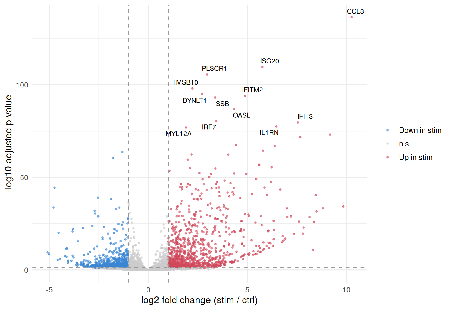
The signature figure for a DE result is the volcano plot — effect size (log2FoldChange) against significance (-log10(padj)) — so you see magnitude and confidence at once. Genes past both a fold-change and an FDR threshold are highlighted, and the strongest ISGs are labelled.
library(Matrix); library(DESeq2); library(ggplot2); library(ggrepel)d <-readRDS("_data/kang_subset.rds")counts <- d$counts; meta <- d$metamono <- meta$cell =="CD14+ Monocytes"cm <- counts[, mono]; mm <- meta[mono, ]sample_id <-paste(mm$ind, mm$stim, sep ="_")pb <-t(rowsum(t(as.matrix(cm)), group = sample_id))si <-unique(data.frame(sample = sample_id, ind = mm$ind, stim = mm$stim))rownames(si) <- si$sample; si <- si[colnames(pb), ]si$ind <-factor(si$ind)si$stim <-factor(si$stim, levels =c("ctrl", "stim"))pb <- pb[rowSums(pb) >=10, ]dds <-DESeq(DESeqDataSetFromMatrix(round(pb), colData = si, design =~ ind + stim), quiet =TRUE)res <-results(dds, contrast =c("stim", "stim", "ctrl"))df <-as.data.frame(res); df$gene <-rownames(df); df <- df[!is.na(df$padj), ]df$dir <-ifelse(df$padj <0.05&abs(df$log2FoldChange) >1,ifelse(df$log2FoldChange >0, "Up in stim", "Down in stim"), "n.s.")top <-head(df[order(df$padj), ], 12)ggplot(df, aes(log2FoldChange, -log10(padj), color = dir)) +geom_point(size =0.7, alpha =0.6) +scale_color_manual(values =c("Up in stim"="#d1495b", "Down in stim"="#3a86d4", "n.s."="grey80"),name =NULL) +geom_text_repel(data = top, aes(label = gene), color ="black", size =3, max.overlaps =20) +geom_vline(xintercept =c(-1, 1), linetype ="dashed", color ="grey60") +geom_hline(yintercept =-log10(0.05), linetype ="dashed", color ="grey60") +labs(x ="log2 fold change (stim / ctrl)", y ="-log10 adjusted p-value") +theme_minimal(base_size =12)
The plot reads at a glance: a tall wall of red on the right — the interferon response, a coordinated up-regulation of many genes — with the ISGs punching highest (both very large fold changes and the smallest p-values). The biology is not subtle, which is exactly why it is such a clean teaching case: a correct method finds a strong, coherent, named signal, not 83% of the transcriptome.
Honest caveats: what pseudobulk needs and where its limits are
Pseudobulk is the right default, but it is not magic. Keep three things straight:
It needs real replication — usually at least 3 donors per condition. Pseudobulk uses the biological replicates you have; it cannot invent them. With one sample per arm (the integration dataset) there is nothing to test, and DESeq2 will refuse or return nothing. If your design has too few replicates, that is an experimental-design problem no statistic can rescue.
It needs enough cells per sample to aggregate. A pseudobulk profile built from a handful of cells is noisy. A common rule of thumb is to require a minimum number of cells (say ~10) per donor-condition-celltype before trusting that pseudobulk sample; drop the cell types where a donor barely contributes any cells.
DESeq2 is one valid engine, not the only one.edgeR and limma-voom are equally accepted on pseudobulk counts and often agree closely. And the muscat package streamlines the entire workflow across all cell types at once — muscat::aggregateData() builds the pseudobulk matrices and pbDS() runs the per-cell-type DE — which is what you will reach for on a real study with a dozen cell types rather than the single one shown here.
Which test when: markers vs cross-condition DE
The per-cell Wilcoxon test is not wrong — it is being used for the wrong question here. Keep the two apart:
Marker genes — use the per-cell test (FindAllMarkers / FindMarkers). “Which genes distinguish cluster 3 from the rest?” is a question about the cells, comparing groups of cells you defined; treating each cell as an observation is appropriate, and this is exactly what the marker-genes lesson does.
Cross-condition DE — use pseudobulk. “Which genes change between conditions within a cell type?” is a question about the samples/donors, so the donors are the replicates and per-cell testing pseudoreplicates. This lesson.
The single distinction: are you comparing cells (markers → per-cell test) or conditions across donors (DE → pseudobulk)? Get that right and you will never inflate an FDR again. This is the same DESeq2 workflow you would run on bulk RNA-seq — see the bulk DESeq2 tutorial for the count-modeling details — with pseudobulk aggregation the one extra step that adapts it to single-cell data.
Common issues
DESeq2 says nearly every gene is significant. You almost certainly fed it per-cell data instead of pseudobulk, or you aggregated but forgot to block on the donor. Aggregate first (rowsum() / AggregateExpression()) so the columns are samples, not cells, and use the ~ ind + stim design. If the column count going into DESeqDataSetFromMatrix() is in the thousands, you did not aggregate.
A ~ ind + stim model with a numeric donor gives a strange result or a warning. DESeq2 is treating the donor ID as a continuous covariate. Convert it: si$ind <- factor(si$ind). The warning “the design formula contains one or more numeric variables … did you mean for this to be a factor?” is the tell.
Few or no differentially expressed genes. Usually too few replicates, or too few cells per sample to aggregate. Check how many donors each condition actually has (table(si$stim)) and how many cells went into each pseudobulk column. Pseudobulk with 2 vs 2 donors has very little power; that is a design limit, not a bug.
Only one sample per condition. Then you cannot do differential expression at all — there is no replication to estimate variability from. Pseudobulk does not help here; you need more samples. (This is why the 2-sample integration dataset was fine for aligning cells but wrong for a condition test.)
Frequently asked questions
NoteWhy is per-cell differential expression (FindMarkers) wrong for comparing conditions?
Because it treats every cell as an independent replicate, but cells from the same donor are not independent — they share that donor’s genetics and batch. Counting cells as replicates (pseudoreplication) inflates the effective sample size from a few donors to thousands of cells, which shrinks p-values and inflates the false discovery rate. On a null comparison with no real signal, a per-cell Wilcoxon test still calls dozens of genes “significant” while pseudobulk correctly calls none.
NoteWhat is pseudobulk differential expression?
Pseudobulk sums the raw counts of all cells from one sample (one donor, within one cell type) into a single expression profile, turning a single-cell experiment back into a bulk-style one with the donors as replicates. You then run a standard bulk RNA-seq method — DESeq2, edgeR, or limma-voom — on those per-donor profiles. It is the field’s recommended method for cross-condition single-cell DE (Squair 2021; Crowell 2020).
NoteHow do I make a pseudobulk matrix in R from a Seurat object?
Use Seurat::AggregateExpression(obj, group.by = c("donor", "condition")), which sums each group’s counts into one column. Without Seurat it is one line of base R on the count matrix: pb <- t(rowsum(t(as.matrix(counts)), group = paste(donor, condition, sep = "_"))). Both give a genes × samples matrix you pass to DESeqDataSetFromMatrix().
NoteHow many replicates do I need for pseudobulk DE?
The donors are your replicates, so you need several per condition — a common minimum is at least 3 per group, and more is better. Pseudobulk cannot create replication you did not collect: with one sample per condition there is no variability to estimate and no valid test. You also want enough cells per donor-condition-celltype (roughly ≥10) so each pseudobulk profile is not dominated by noise.
NoteShould I use DESeq2, edgeR, or limma-voom for pseudobulk?
All three are valid on pseudobulk counts and usually agree closely; DESeq2 and edgeR model the counts directly, limma-voom transforms them first. Pick the one you know. For a real study with many cell types, the muscat package wraps the whole workflow (aggregateData() + pbDS()) so you run pseudobulk DE across every cell type at once instead of one at a time.
Test your understanding
ImportantYour turn: run pseudobulk DE on the B cells
Repeat the workflow, but on the B cells instead of the monocytes. Subset to meta$cell == "B cells", aggregate to one pseudobulk profile per donor per condition, run DESeq2 with the design ~ ind + stim (remember factor(ind)), and report how many genes are significant at 5% FDR. Are the top hits still interferon-stimulated genes?
TipHint
The only change from the monocyte code is the subset line: bcell <- meta$cell == "B cells". Everything downstream — paste(ind, stim), rowsum(), factor(ind), the ~ ind + stim design, the stim vs ctrl contrast — is identical. Count with sum(res$padj < 0.05, na.rm = TRUE) and read the top rows with head(res[order(res$padj), ]).
TipSolution
library(Matrix); library(DESeq2)d <-readRDS("_data/kang_subset.rds")counts <- d$counts; meta <- d$metabcell <- meta$cell =="B cells"cm <- counts[, bcell]; mm <- meta[bcell, ]sample_id <-paste(mm$ind, mm$stim, sep ="_")pb <-t(rowsum(t(as.matrix(cm)), group = sample_id))si <-unique(data.frame(sample = sample_id, ind = mm$ind, stim = mm$stim))rownames(si) <- si$sample; si <- si[colnames(pb), ]si$ind <-factor(si$ind)si$stim <-factor(si$stim, levels =c("ctrl", "stim"))pb <- pb[rowSums(pb) >=10, ]dds <-DESeq(DESeqDataSetFromMatrix(round(pb), si, design =~ ind + stim), quiet =TRUE)res <-results(dds, contrast =c("stim", "stim", "ctrl"))sum(res$padj <0.05, na.rm =TRUE) # significant genes at 5% FDRhead(res[order(res$padj), ]) # top hits — still ISGs (ISG20, ISG15, LY6E, ...)
B cells mount the same interferon program: the workflow is unchanged, and the top of the list is again dominated by interferon-stimulated genes. That reproducibility across cell types is the biology — every cell type responds to IFN-β, so a correct method finds the same ISG signature in each.
NoteQuick check: your pseudobulk matrix has 2,400 columns and DESeq2 flags 80% of genes as significant. What went wrong?
A. Nothing — a real interferon response can hit 80% of genes. B. You never aggregated: 2,400 columns means the matrix is still one column per cell, so DESeq2 is pseudoreplicating just like FindMarkers. C. You used the wrong contrast direction.
TipShow answer
B. A pseudobulk matrix should have one column per sample (donor × condition) — here that is 16, not 2,400. Thousands of columns means you passed the per-cell matrix straight to DESeq2 without summing, so it is treating cells as replicates and the inflated significance is the pseudoreplication artifact this lesson exists to prevent. Aggregate with rowsum() / AggregateExpression() first.
Conclusion
Cross-condition differential expression in single-cell data has a right way and a wrong way, and the difference is which unit you treat as a replicate. The wrong way — a per-cell test like FindMarkers — counts thousands of cells as thousands of samples, pseudoreplicates, and inflates the FDR so badly it invents dozens of hits from pure noise. The right way is pseudobulk: sum each donor’s cells into one profile, then run DESeq2 (or edgeR / limma-voom) with the design ~ donor + condition and the donor as a factor, so the condition effect is estimated across genuine biological replicates. On the Kang IFN-β monocytes that gives a strong, interpretable result — 2,275 genes, led by the canonical interferon-stimulated genes — that will survive review. Remember the one distinction that decides the method: comparing cells is a marker question (per-cell test); comparing conditions across donors is a DE question (pseudobulk).
Ask Prova“how do I run pseudobulk differential expression on my own multi-sample Seurat object with DESeq2?” — it answers with R code you can run on your own data: aggregate each donor’s cells with AggregateExpression(), build the colData, fit DESeq2 with the donor as a blocking factor, and read the result — instead of pseudoreplicating with FindMarkers. The runtime is the judge.Ask Prova →
Was this page helpful?
Thanks for the feedback!
Prove you can do it. Master the whole Single-Cell RNA-Seq Analysis in R series — track your path, build projects, and earn a certificate.
This lesson is reproducible: every figure and number was produced by the code shown — copy any block and run it to reproduce them. The runtime is the judge.
Crowell, H. L., et al. (2020). muscat detects subpopulation-specific state transitions from multi-sample multi-condition single-cell transcriptomics data. Nature Communications, 11, 6077. https://www.nature.com/articles/s41467-020-19894-4
Murphy, A. E., & Skene, N. G. (2022). A balanced measure shows superior performance of pseudobulk methods in single-cell RNA-sequencing analysis. Nature Communications, 13, 7851. https://www.nature.com/articles/s41467-022-35519-4
Kang, H. M., et al. (2018). Multiplexed droplet single-cell RNA-sequencing using natural genetic variation — the source of the Kang IFN-β PBMC dataset. Nature Biotechnology, 36(1), 89–94. https://www.nature.com/articles/nbt.4042