Monocle3 Trajectory Analysis in R: Pseudotime with a Principal Graph
Learn a principal graph on your cells with Monocle3, root and order pseudotime with learn_graph and order_cells, and find dynamic genes with graph_test — the graph-based contrast to Slingshot
Bioinformatics
A practical guide to trajectory inference and pseudotime with Monocle3 in R. Build a cell_data_set, learn a principal graph directly on Monocle3’s own UMAP, root and order the cells with learn_graph and order_cells, and test which genes change along the graph with graph_test (Moran’s I). See how Monocle3’s partitions honestly split disconnected cells off the trajectory — the graph-based counterpart to Slingshot’s minimum spanning tree — on the canonical Nestorowa mouse blood stem/progenitor dataset.
Published
July 4, 2026
Modified
July 7, 2026
TipKey takeaways
Monocle3 learns a graph, not a tree of cluster centres. It fits a principal graph — a smooth skeleton of nodes and edges — directly through the cells with reversed graph embedding (RGE), so the trajectory can branch, converge, or even loop, and it is drawn on Monocle3’s own UMAP (uniform manifold approximation and projection) (Cao et al., 2019). This is the contrast with Slingshot, which builds a minimum spanning tree on cluster centroids and smooths principal curves.
The pipeline is one ordered sequence of verbs.preprocess_cds() (principal component analysis) → reduce_dimension() (UMAP) → cluster_cells() (clusters and partitions) → learn_graph() (the principal graph) → order_cells() (pseudotime from a root you choose).
Partitions are Monocle3’s honest “these cells are not connected” call.cluster_cells() also splits cells into partitions — groups it judges to be separate manifolds — and learn_graph() fits a graph within each. Cells in a disconnected partition get infinite pseudotime: Monocle3 refuses to invent a path where the data does not show one. That is a feature, and you can override it with learn_graph(use_partition = FALSE) when you believe it really is one continuum.
Root the graph programmatically, not by clicking.order_cells() wants a starting principal-graph node. The interactive picker is fine for exploring, but for a reproducible script pass root_pr_nodes = the node nearest your known origin — here the long-term stem cells.
graph_test() finds dynamic genes with Moran’s I. Instead of fitting a curve per lineage, Monocle3 tests each gene for spatial autocorrelation over the graph (Moran’s I): do nearby cells on the trajectory share similar expression? Genes that do are the ones changing along it.
Introduction
You have clustered a single-cell RNA-seq (scRNA-seq) dataset and you can see it is not a set of tidy islands — the cells run together into a connected, branching shape. That is a differentiating population, and the question is no longer “what type is each cell?” but “how far along its developmental path is each cell, and which genes drive it there?” The Slingshot lesson answers that with a minimum spanning tree on cluster centroids and smooth principal curves. This lesson answers it with Monocle3, which takes a different route to the same goal — and the differences are worth understanding, because they change what the trajectory can express and how honest it is about cells that do not belong on it.
Monocle3 does not summarize the cells into cluster centres and connect those. It learns a principal graph: a network of nodes and edges fitted through the cells themselves with reversed graph embedding (RGE) — the idea of simultaneously embedding the data and a graph that runs along its backbone, introduced for single-cell trajectories in Monocle 2 (Qiu et al., 2017) and scaled to large, UMAP-based datasets in Monocle3 (Cao et al., 2019). A graph can branch and converge freely, so Monocle3 handles complex topologies a simple tree cannot. And it is candid about structure: if two groups of cells are not connected, it says so and keeps them apart.
We work on the same dataset as the Slingshot lesson so you can compare the two methods on identical cells: the canonical Nestorowa mouse blood dataset (Nestorowa et al., 2016), 1,920 hematopoietic stem and progenitor cells (HSPCs — the stem and progenitor cells that produce every blood cell). Each cell carries a FACS label (fluorescence-activated cell sorting — the flow-cytometry gating that sorted cells by surface markers) recording which progenitor population it belongs to. We never feed those labels to Monocle3; we hold them back to check the trajectory it infers.
How Monocle3 differs from Slingshot
Both tools order cells along a differentiation continuum and give you a pseudotime — a single number per cell measuring how far it has progressed, low at the start and high at the committed end. But they build the trajectory in genuinely different ways, and that shapes what you get.
Slingshot
Monocle3
What it fits
A minimum spanning tree (MST) on cluster centroids, smoothed into principal curves
A principal graph learned through the cells with reversed graph embedding
Runs on
Your embedding (e.g. the Seurat UMAP) + your cluster labels
Its own UMAP, built inside the cell_data_set
Topology
A tree (branches from a root, no loops)
A graph — can branch, converge, or loop
Disconnected cells
Forced into the tree; every cell gets a pseudotime
Split into partitions; cells off the main graph get infinite pseudotime
Dynamic-gene test
tradeSeq — a GAM of expression vs pseudotime per lineage
graph_test() — Moran’s I spatial autocorrelation over the graph
The practical upshot: Slingshot is the clean, robust default when you already have a good embedding and a clear branching tree. Monocle3 is the tool to reach for when the topology is more complex, or when you want the method to tell you which cells form a connected trajectory rather than forcing them all onto one — as you are about to see it do.
The data: stem cells with known progenitor labels
The committed nestorowa_hsc.rds is a slice of the Nestorowa HSPC atlas — the same file the Slingshot lesson uses. It holds a raw count matrix of 2,500 genes across 1,920 cells, a metadata table, and a symbol map from Ensembl gene IDs to readable gene names. The broad column records the FACS population each cell was sorted into — LTHSC (long-term hematopoietic stem cell, LT-HSC — the apex stem cell), MPP (multipotent progenitor), LMPP (lymphoid-primed multipotent progenitor), CMP (common myeloid progenitor), GMP (granulocyte-macrophage progenitor — the myeloid fate), and MEP (megakaryocyte-erythroid progenitor — the red-cell / platelet fate), plus a group of cells with no fine label. That gradient from stem cell to committed progenitor is the differentiation ground truth we validate the trajectory against.
Monocle3 does not work on a Seurat object; it works on a cell_data_set (a CDS — Monocle3’s container built on Bioconductor’s SingleCellExperiment). Build it from three pieces: the count matrix, a cell-metadata table, and a gene-metadata table whose gene_short_name column Monocle3 uses to label genes on plots.
library(monocle3)d <-readRDS("_data/nestorowa_hsc.rds")# Gene metadata: Monocle3 labels plots from a `gene_short_name` columngene_meta <-data.frame(gene_short_name = d$symbol[rownames(d$counts)],row.names =rownames(d$counts))cds <-new_cell_data_set(d$counts,cell_metadata = d$meta,gene_metadata = gene_meta)cds
That prints the CDS dimensions — 2,500 genes by 1,920 cells — and the counts per sorted population, from the LT-HSC apex down to the committed GMP and MEP progenitors, plus the unlabelled cells.
Note
The blocks in this lesson build one Monocle3 object step by step, so run them in order in a single session — each verb (preprocess_cds, reduce_dimension, …) adds to the cds the previous block created. The full pipeline is a fixed pattern you will reuse verbatim: only the arguments change.
Preprocess, embed, and cluster
Monocle3 runs its own dimension-reduction pipeline on the CDS. Three verbs do it. preprocess_cds() runs principal component analysis (PCA) — a linear reduction that keeps the top directions of variation; we keep 30 components. reduce_dimension() then builds a UMAP (the non-linear 2-D map) from those components. cluster_cells() groups the cells — and, importantly, also assigns partitions: coarser groupings of cells it judges to sit on separate manifolds. We set a seed before each step because PCA, UMAP, and clustering all use randomness, and a trajectory built on shifting clusters is not reproducible.
set.seed(42); cds <-preprocess_cds(cds, num_dim =30) # PCAset.seed(42); cds <-reduce_dimension(cds, reduction_method ="UMAP")set.seed(42); cds <-cluster_cells(cds)length(unique(partitions(cds))) # how many separate manifolds Monocle3 found
[1] 2
length(unique(clusters(cds))) # how many clusters
[1] 2
table(partition =partitions(cds)) # cells per partition
partition
   1    2
1138  782
Monocle3 splits these cells into two partitions — 1,138 cells in one and 782 in the other — and finds two clusters. Read that split carefully: Monocle3 is telling you it does not see these 1,920 cells as one connected manifold. It has decided the 782-cell group is separate enough that a single trajectory through all the cells would be dishonest. Hold that thought — it drives everything below, and it is the sharpest difference from Slingshot, which forced every cell into one connected tree.
Learn the principal graph
Now the heart of Monocle3: learn_graph() fits the principal graph — the smooth skeleton of nodes (called principal points, named Y_1, Y_2, …) and edges that runs along the backbone of the cells. This is the reversed-graph-embedding step: the graph and the cells are fitted together so the graph traces the trajectory through the data (Cao et al., 2019). By default learn_graph() fits a separate graph within each partition, so the disconnected 782-cell group gets its own skeleton rather than being wired to the main one.
# learn_graph() prints a progress bar while it fits the graph; there is no# result to show (the graph is stored inside the CDS), so we silence the output.cds <-learn_graph(cds)
There is no printed output — the graph is stored inside the CDS. You will see it in a moment, drawn over the cells.
Root and order the cells
A graph on its own has no direction. order_cells() turns it into a pseudotime, but it needs a root: the principal-graph node where time starts. Monocle3 offers an interactive picker (order_cells(cds) with no root opens a plot you click), which is convenient for exploring but not reproducible — a script must not depend on a mouse click. Instead, find the root programmatically: locate the principal node closest to the cells you know are the origin. Here that is the LT-HSC stem cells, read from the FACS broad label.
The helper below is the pattern from the Monocle3 documentation: for the cells of a chosen type, find the graph node each is projected onto, and take the node that the most of them map to.
# The principal node nearest the LT-HSC stem cells = the biological rootget_earliest_root <-function(cds, cell_col, target) { cell_ids <-which(colData(cds)[[cell_col]] == target) closest <-principal_graph_aux(cds)[["UMAP"]]$pr_graph_cell_proj_closest_vertex igraph::V(principal_graph(cds)[["UMAP"]])$name[as.numeric(names(which.max(table(closest[cell_ids, ]))))]}root_node <-get_earliest_root(cds, "broad", "LTHSC")root_node
sum(is.finite(pt)) # how many cells got a pseudotime
[1] 1138
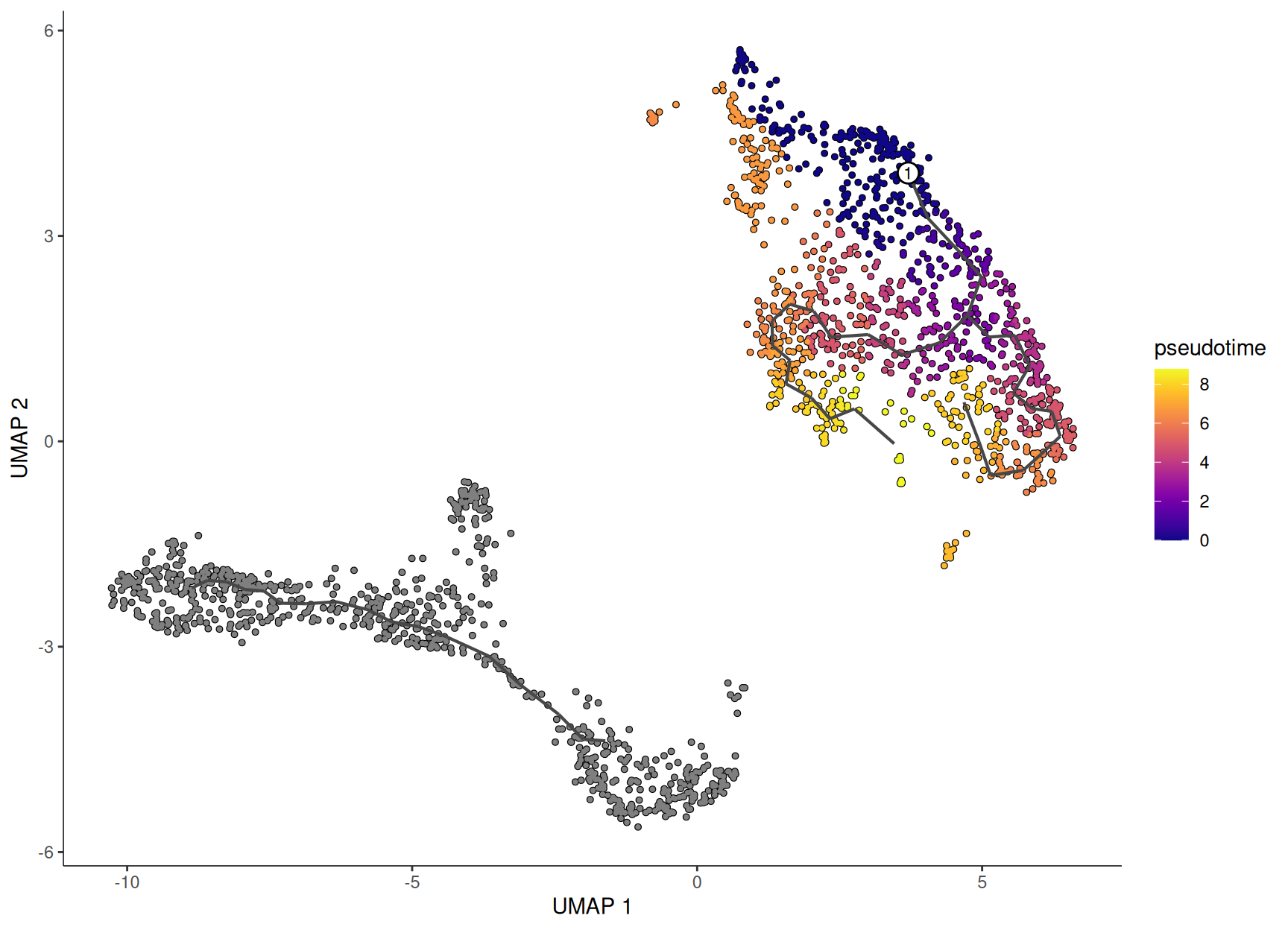
The stem cells anchor the root at node Y_3, and pseudotime runs from 0 at the root to about 8.8 at the far end of the graph. But look at the count: only 1,138 of the 1,920 cells have a finite pseudotime. The other 782 — exactly the second partition — are at infinite pseudotime, because they sit on a graph disconnected from the root. Monocle3 will not order cells it cannot reach from the start. pseudotime() returns Inf for them by design; downstream you filter to the finite cells.
See the trajectory: the graph coloured by pseudotime
plot_cells() is Monocle3’s one-stop plotting verb. Colour the cells by pseudotime and it lays the principal graph over the UMAP with the pseudotime gradient underneath — dark at the root, bright at the tips. The disconnected partition, with no pseudotime, shows in grey.
The principal graph threads through the main body of cells, rooted in the dark stem-cell region and brightening outward as cells mature — the differentiation gradient, drawn as a graph rather than as separate curves. The grey block is the second partition: Monocle3 built it a graph of its own but never connected it to the root, so those cells carry no pseudotime. That honesty — these cells are not on this trajectory — is exactly what partitions buy you.
Validate the graph against the known labels
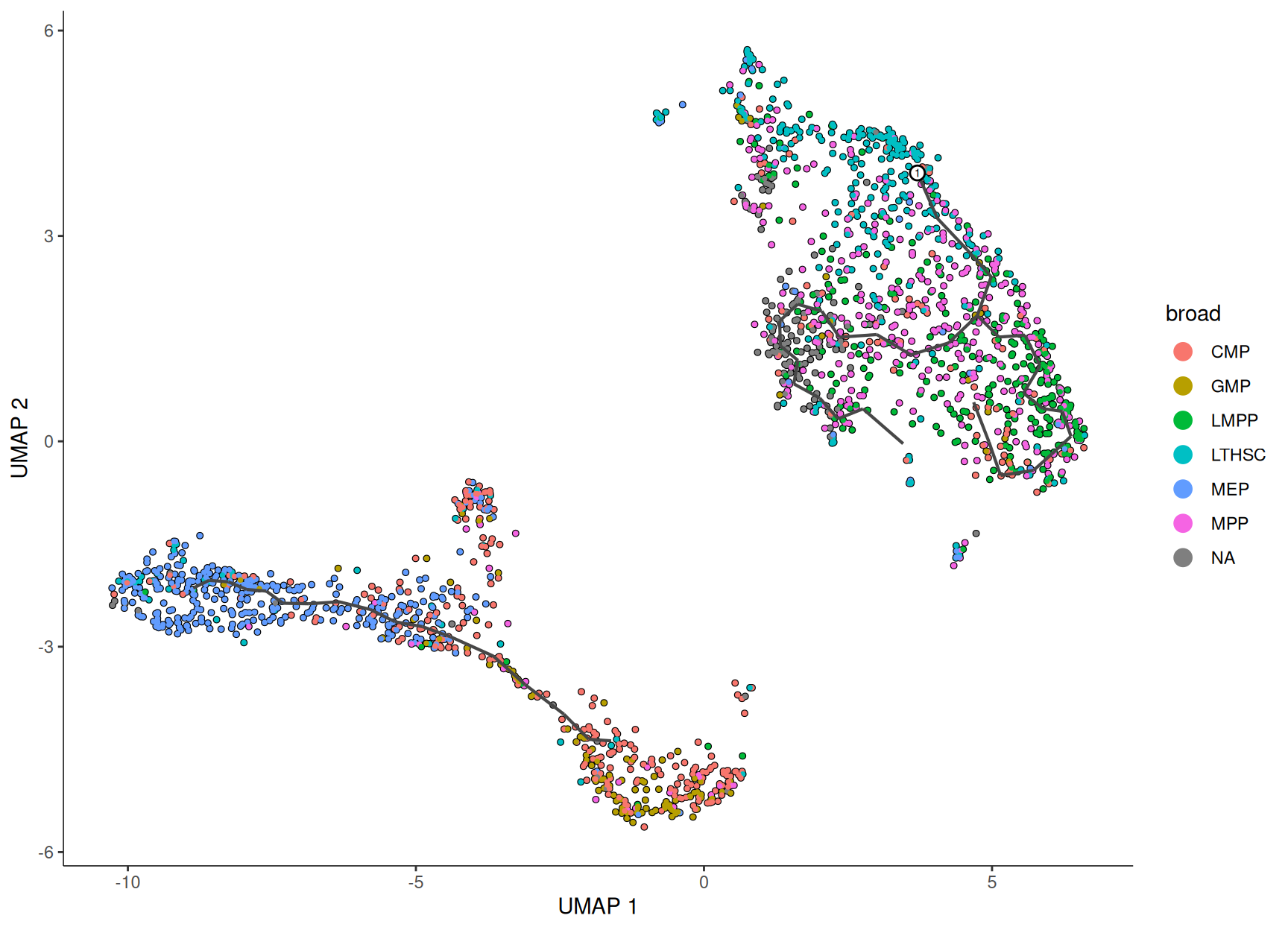
A trajectory that looks plausible still has to match the biology you held back. Colour the same plot by the FACS broad label: the rooted, low-pseudotime end of the graph should sit on the stem cells, and the graph should run out toward the committed progenitors.
The root end of the graph sits squarely on the LTHSC stem cells, and the graph runs out through the progenitor populations toward the committed fates — Monocle3 placed the stem cells at the start of pseudotime without ever seeing the FACS labels. That agreement between the inferred trajectory and the known sorting is your evidence it is real, not an artifact of the embedding.
Find genes that change along the graph with graph_test()
Pseudotime is a means; the payoff is which genes drive the differentiation. Monocle3 answers this with graph_test(), and it uses a different statistic from tradeSeq. Rather than fitting a curve of expression against pseudotime per lineage, it computes Moran’s I — a measure of spatial autocorrelation — for each gene over the principal graph. Moran’s I asks a simple question: do cells that are neighbours on the graph tend to have similar expression of this gene? A gene that switches on in one region and off in another is highly autocorrelated (high Moran’s I); a gene scattered randomly across the graph is not. High-Moran’s-I genes are the ones whose expression is organized by the trajectory.
We run it once, on the principal graph. graph_test() prints a long per-gene progress bar while it works, so we compute it in a quiet chunk (output hidden) and read off the significant genes in the next block.
Of the 2,500 genes tested, 1,372 are significant at a 5% false-discovery rate (q_value) — a large fraction, as expected in a population whose whole reason for existing is to differentiate. The top of the list, ranked by Moran’s I, is a roll-call of canonical blood-lineage markers, and they sort cleanly by fate:
Erythroid (red-cell):Klf1, Car1, Rhd — the master erythroid transcription factor and its downstream program.
Myeloid (granulocyte):Mpo, Prtn3, Ctsg — the neutrophil granule enzymes.
Lymphoid:Ighm, Dntt — immunoglobulin and the lymphoid-progenitor marker terminal transferase.
That the strongest spatially-organized genes are exactly the known fate markers is the biological confirmation that graph_test() found real structure, not noise — the same genes tradeSeq surfaces on this data by a completely different statistic.
Plot dynamic genes on the graph
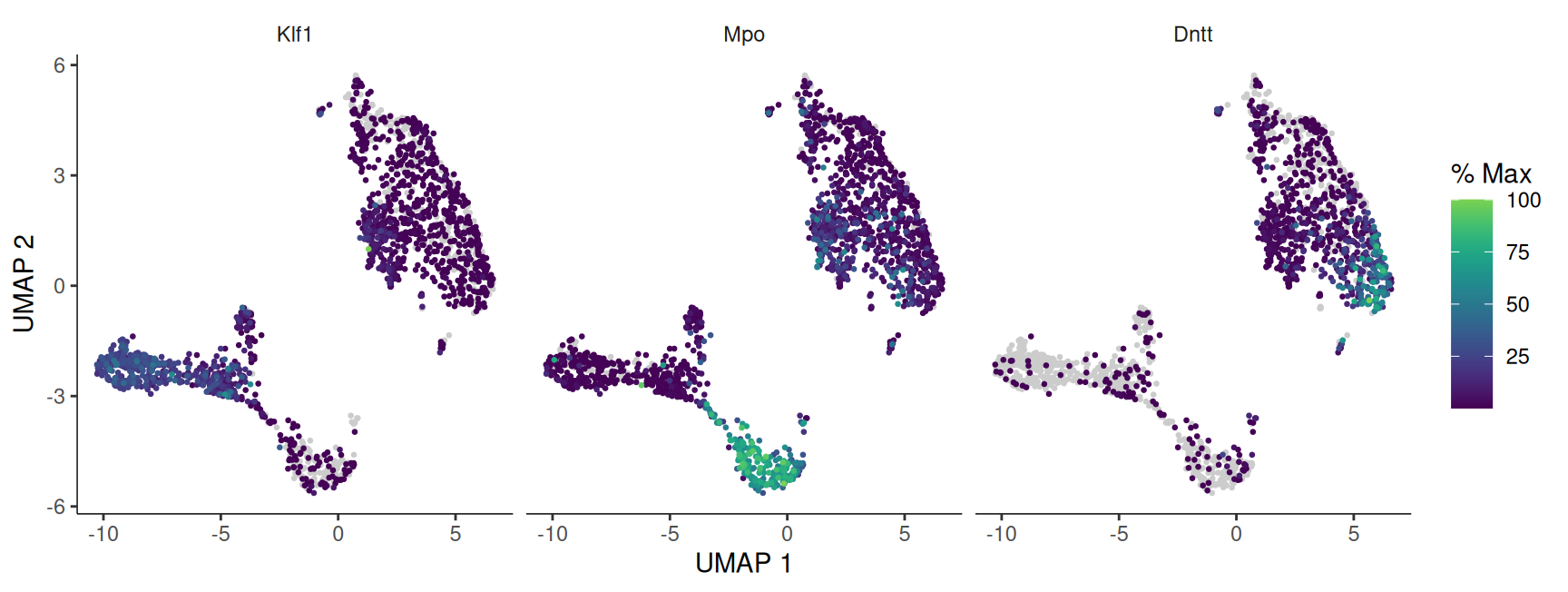
The clearest way to see a dynamic gene is to paint its expression onto the graph. Pass plot_cells() a few genes and it facets one UMAP per gene, colouring cells by expression. Pick one marker per fate — erythroid, myeloid, lymphoid — and each should light up in a different region of the graph, tracking where that fate commits.
Each marker is high in its own part of the graph and quiet elsewhere: the erythroid gene Klf1, the myeloid granule gene Mpo, and the lymphoid gene Dntt each mark a different arm. The principal graph has separated the committing lineages, and graph_test() picked exactly the genes that distinguish them — the whole point of the analysis, in one figure.
The partition question: one trajectory or two?
Come back to those two partitions, because this is the decision Monocle3 hands you that Slingshot does not. Monocle3 judged the 782-cell group disconnected and gave it infinite pseudotime. Sometimes that is right — the cells really are a separate population (a contaminating cell type, a distinct manifold). Sometimes it is too cautious — you have biological reason to believe it is all one continuum and the gap is a sampling or embedding artifact.
When you believe it is one trajectory, override the default with learn_graph(use_partition = FALSE), which fits a single graph across all partitions. Re-root and re-order, and every cell gets a finite pseudotime.
# learn_graph() again prints a progress bar; compute quietly, read the result below.cds_one <-learn_graph(cds, use_partition =FALSE)cds_one <-order_cells(cds_one,root_pr_nodes =get_earliest_root(cds_one, "broad", "LTHSC"))
pt_one <-pseudotime(cds_one)range(pt_one[is.finite(pt_one)]) # pseudotime scale with one connected graph
[1] 0.00000 22.81901
sum(is.finite(pt_one)) # now every cell is ordered
[1] 1920
With one connected graph, all 1,920 cells get a finite pseudotime and the scale stretches to about 22.8 — the graph now spans both former partitions. Which is right? That is a biological judgement, not a default to accept blindly: if the FACS labels and marker genes say the two partitions are one differentiating continuum, use_partition = FALSE is the honest choice; if the second group is a genuinely distinct population, leave the partitions in place and keep it off the trajectory. Monocle3’s contribution is to surface the question rather than silently answer it for you.
Which method when
You have…
Use
Why
A clear branching differentiation in R, with a good embedding already
Slingshot and Monocle3 are not rivals so much as complements: run both on a hard dataset and where they agree you can trust the trajectory; where they disagree — most often about whether cells form one continuum or several — Monocle3’s partitions tell you why.
Common issues
order_cells() opens an interactive plot and my script stalls. Called as order_cells(cds) with no root, Monocle3 launches a click-to-pick-root widget — fine interactively, but it blocks a non-interactive render or script. Always pass a root explicitly: order_cells(cds, root_pr_nodes = "Y_3"), or compute the node from a known cell type with the get_earliest_root() helper above. A reproducible pipeline never depends on a mouse click.
Most of my cells have infinite pseudotime. They are in a partition disconnected from the root. Monocle3 only orders cells reachable from the start node, so cells on a separate graph get Inf. Decide whether that is correct: if the extra cells are a genuinely distinct population, filter to is.finite(pseudotime(cds)) and move on; if you believe it is all one continuum, refit with learn_graph(cds, use_partition = FALSE) to span the partitions, then re-root and re-order.
I have a Seurat object, not a cell_data_set. Monocle3 needs a CDS. Either rebuild one from the raw pieces with new_cell_data_set(counts, cell_metadata, gene_metadata) as in this lesson (the most robust route, independent of Seurat versions), or convert directly with SeuratWrappers::as.cell_data_set(seurat_obj). If you convert, re-run cluster_cells() and learn_graph() on the CDS — Monocle3 needs its own clusters and partitions to build the graph.
Frequently asked questions
NoteWhat is Monocle3 trajectory analysis?
Monocle3 infers a developmental trajectory by learning a principal graph — a smooth skeleton of nodes and edges — directly through your cells in a low-dimensional space, then ordering the cells along it to give each a pseudotime. Unlike a method that connects cluster centres with a tree, its graph can branch, converge, or loop, so it handles more complex topologies. You run it as a pipeline: preprocess_cds() → reduce_dimension() → cluster_cells() → learn_graph() → order_cells().
NoteMonocle3 vs Slingshot — which should I use?
Slingshot fits a minimum spanning tree on cluster centroids and smooth principal curves on your embedding — simple, robust, Seurat-native, and ideal for a clear branching tree. Monocle3 learns a principal graph on its own UMAP, handles disconnected cells with partitions (giving them infinite pseudotime rather than forcing a path), and tests dynamic genes with Moran’s I via graph_test(). Use Slingshot for a straightforward tree; reach for Monocle3 for complex or possibly-disconnected topologies, or when you want the method to flag cells that are not on the trajectory.
NoteHow do I set the root for pseudotime in Monocle3?
Pass order_cells() a starting node of the principal graph via root_pr_nodes. Rather than clicking the interactive picker (which is not reproducible), compute the node nearest a known origin cell type: find the principal node most of your stem cells project onto, then order_cells(cds, root_pr_nodes = that_node). Rooting from biological knowledge — a stem-cell marker or a FACS label — is what makes the pseudotime direction meaningful.
NoteWhy do so many cells have infinite pseudotime?
Because they are in a partition that is disconnected from the root. cluster_cells() splits cells into partitions — groups it judges to be separate manifolds — and learn_graph() fits a graph within each. Cells not reachable from the root node get Inf pseudotime by design; Monocle3 will not invent a path across a gap. If you believe the cells really are one continuum, refit with learn_graph(cds, use_partition = FALSE) to span all partitions with a single graph.
NoteHow does graph_test find genes that change along the trajectory?
graph_test(cds, neighbor_graph = "principal_graph") computes Moran’s I, a spatial-autocorrelation statistic, for each gene over the principal graph. It asks whether cells that are neighbours on the trajectory have similar expression: a gene that is high in one region and low in another scores a high Moran’s I, while a randomly scattered gene scores near zero. The genes significant at your chosen false-discovery rate (the q_value column) are the ones whose expression is organized by the trajectory.
Test your understanding
ImportantYour turn: fit the trajectory with and without partitions
Using nestorowa_hsc.rds, build the cell_data_set, run the full pipeline (preprocess_cds → reduce_dimension → cluster_cells → learn_graph → order_cells, rooted at the LT-HSC–enriched node), and record how many cells get a finite pseudotime. Then refit the graph with learn_graph(cds, use_partition = FALSE), re-root, re-order, and record the count again. How many cells does each version order, and what does the difference tell you about the second partition?
TipHint
The only change between the two runs is the use_partition argument to learn_graph(). Count ordered cells with sum(is.finite(pseudotime(cds))) after each order_cells(). Re-use the get_earliest_root() helper to root both versions the same way, so the only thing that differs is whether the graph spans the partitions.
TipSolution
library(monocle3)d <-readRDS("_data/nestorowa_hsc.rds")gene_meta <-data.frame(gene_short_name = d$symbol[rownames(d$counts)],row.names =rownames(d$counts))cds <-new_cell_data_set(d$counts, cell_metadata = d$meta, gene_metadata = gene_meta)set.seed(42); cds <-preprocess_cds(cds, num_dim =30)set.seed(42); cds <-reduce_dimension(cds, reduction_method ="UMAP")set.seed(42); cds <-cluster_cells(cds)get_earliest_root <-function(cds, cell_col, target) { cell_ids <-which(colData(cds)[[cell_col]] == target) closest <-principal_graph_aux(cds)[["UMAP"]]$pr_graph_cell_proj_closest_vertex igraph::V(principal_graph(cds)[["UMAP"]])$name[as.numeric(names(which.max(table(closest[cell_ids, ]))))]}# Default: a graph per partitioncds <-learn_graph(cds)cds <-order_cells(cds, root_pr_nodes =get_earliest_root(cds, "broad", "LTHSC"))sum(is.finite(pseudotime(cds))) # ~1138 of 1920 — the main partition only# One graph across all partitionscds1 <-learn_graph(cds, use_partition =FALSE)cds1 <-order_cells(cds1, root_pr_nodes =get_earliest_root(cds1, "broad", "LTHSC"))sum(is.finite(pseudotime(cds1))) # 1920 — every cell ordered
The default orders about 1,138 cells and leaves the 782-cell second partition at infinite pseudotime; with use_partition = FALSE, all 1,920 cells are ordered. The gap is the second partition. Whether ordering it is correct is a biological call: check whether those cells share the differentiation program (by FACS label and marker genes) before you decide to bridge the gap.
NoteQuick check: Monocle3 gives 782 of your cells infinite pseudotime. What does that mean?
A. The analysis failed — every cell should get a pseudotime. B. Those cells are in a partition disconnected from the root, so Monocle3 will not order them along a graph it cannot reach them on; you decide whether to bridge the gap (use_partition = FALSE) or treat them as a separate population. C. Those cells are the most differentiated, so they sit at the maximum of pseudotime.
TipShow answer
B. Infinite pseudotime marks cells in a partition Monocle3 judged disconnected from the rooted graph. It is not a failure — it is Monocle3 declining to invent an ordering across a gap in the data. The right response is a biological judgement: if those cells belong to the same continuum, refit with learn_graph(use_partition = FALSE) to span the partitions; if they are a genuinely distinct population, filter to the finite-pseudotime cells and analyse them separately.
Conclusion
Monocle3 takes a graph-based route to the same goal as Slingshot: it learns a principal graph through the cells with reversed graph embedding, orders them along it from a root you choose, and gives each a pseudotime. On the Nestorowa blood dataset it rooted the graph in the LT-HSC stem cells — confirmed against the held-back FACS labels — and graph_test() surfaced the canonical erythroid, myeloid, and lymphoid markers by Moran’s I. The defining difference from Slingshot is honesty about structure: Monocle3 split the cells into partitions and gave 782 of them infinite pseudotime rather than force a path, handing you — not hiding — the decision of whether they belong on one trajectory. Run it when your topology is complex or you suspect disconnected populations; run Slingshot for a clean branching tree; and when a dataset is hard, run both and trust the trajectory where they agree.
Related lessons
Trajectory & pseudotime with Slingshot — the tree-based counterpart to this lesson; fits an MST on cluster centroids and smooth curves, and finds dynamic genes with tradeSeq. Read both to choose between them. · Clustering & UMAP — builds the clusters and embedding a trajectory is fitted on; good clusters make a good graph. · Marker genes & cell-type annotation — the discrete counterpart: label stable cell types, the question trajectory analysis does not answer. · Bioinformatics — the pillar.
Where this fits:clustering & UMAP → marker genes & annotation → trajectory & pseudotime (this lesson with Monocle3, or Slingshot) → genes-along-the-graph with graph_test — from a static map of cell types to the dynamic path between them.
🟢 With an AI agent
Ask Prova“how do I run a Monocle3 trajectory on my own Seurat object — build a cell_data_set, learn the graph, set the root programmatically, and find dynamic genes with graph_test?” — it answers with R code you can run on your own data: convert or rebuild the CDS, run the preprocess → reduce → cluster → learn_graph → order_cells pipeline, root it from a known cell type, and test genes with Moran’s I. The runtime is the judge.Ask Prova →
Was this page helpful?
Thanks for the feedback!
Prove you can do it. Master the whole Single-Cell RNA-Seq Analysis in R series — track your path, build projects, and earn a certificate.
This lesson is reproducible: every figure and number was produced by the code shown, run top to bottom in the datanovia/quarto-bioinformatics render image (monocle3 1.4.27) — copy the blocks and run them in order to reproduce them. The committed _freeze is what the site serves. The runtime is the judge.
References
Cao, J., et al. (2019). The single-cell transcriptional landscape of mammalian organogenesis — the Monocle3 method. Nature, 566, 496–502. https://doi.org/10.1038/s41586-019-0969-x
Trapnell, C., et al. (2014). The dynamics and regulators of cell fate decisions are revealed by pseudotemporal ordering of single cells (the original Monocle: pseudotemporal ordering). Nature Biotechnology, 32, 381–386. https://doi.org/10.1038/nbt.2859
Nestorowa, S., et al. (2016). A single-cell resolution map of mouse hematopoietic stem and progenitor cell differentiation — the source of the HSPC dataset. Blood, 128(8), e20–e31. https://doi.org/10.1182/blood-2016-05-716480