Seurat Marker Genes & Cell-Type Annotation in R (pbmc3k)
Find the genes that define each cluster with FindAllMarkers, read canonical PBMC markers off the UMAP, and assign biological cell-type labels to produce an annotated UMAP
Bioinformatics
A practical guide to finding marker genes and annotating cell types in single-cell RNA-seq data with Seurat. Starting from a clustered pbmc3k object, run FindAllMarkers to get the genes that distinguish each cluster, visualize canonical PBMC markers with FeaturePlot and VlnPlot, reason from those markers to a cell-type label for every cluster, relabel with RenameIdents, and produce the annotated UMAP you put in a paper.
Published
June 29, 2026
Modified
July 7, 2026
TipKey takeaways
Clusters 0–8 are unnamed groups of similar cells. FindAllMarkers() finds the genes each cluster over-expresses versus all the others — the statistical evidence you annotate from.
Run it positive-only and lightly filtered: FindAllMarkers(only.pos = TRUE, min.pct = 0.25, logfc.threshold = 0.25) (a Wilcoxon test per gene per cluster). Sort by avg_log2FC for each cluster’s strongest markers.
Annotate by matching markers to known cell types. Plot canonical PBMC markers on the UMAP with FeaturePlot() / VlnPlot() and read which cluster lights up: IL7R → CD4 T, CD14/LYZ → monocytes, MS4A1 → B, CD8A → CD8 T, GNLY/NKG7 → NK, FCER1A → dendritic cells, PPBP → platelets.
RenameIdents() turns the cluster numbers into cell-type names; the relabelled DimPlot() is the signature figure of the whole analysis.
Be honest about what markers can and cannot resolve. Naive vs memory CD4 T is a genuinely subtle split, and the rare clusters (DC, platelet) rest on a single strong marker — label them, but say so.
Introduction
Clustering gave you nine groups, labelled 0 through 8. Those numbers are arbitrary: cluster 0 is “684 cells the graph placed together,” not “T cells.” This lesson does the interpretive work that makes the analysis useful — it names the clusters. The logic is simple and is the same every immunologist uses at the bench: find the genes that are switched on in one cluster and off in the rest, recognize those genes as the markers of a known cell type, and label the cluster accordingly.
Two steps do it. First, FindAllMarkers() computes, for every cluster, the genes that distinguish it from all other cells — the data-driven evidence. Second, you map markers to identities by checking a short list of canonical PBMC markers against the clusters and reasoning from biology to a name. We pick up from the clustering lesson on the same pbmc3k object, so the workflow transfers directly to your own clustered data.
Pick up from C4: rebuild the clustered object
Each code block here is self-contained, so it starts by re-creating the clustered object from the previous lesson — load the 10x matrix, build the Seurat object, QC-filter, normalize, find variable features, scale, run PCA, build the neighbor graph, cluster at resolution 0.5, and run UMAP. This is exactly the object you ended C4 with: 2,638 cells in 9 clusters.
Modularity Optimizer version 1.3.0 by Ludo Waltman and Nees Jan van Eck

Number of nodes: 2638
Number of edges: 95927

Running Louvain algorithm...
Maximum modularity in 10 random starts: 0.8728
Number of communities: 9
Elapsed time: 0 seconds
pbmc <-RunUMAP(pbmc, dims =1:10)table(Idents(pbmc)) # 9 clusters, largest first
Nine clusters, 684 cells down to 13. Everything below runs on this object.
Find marker genes for every cluster
A marker gene for a cluster is a gene expressed much more in that cluster than in the rest of the cells. FindAllMarkers() finds them by testing, one cluster at a time, each gene’s expression in that cluster against all other cells with a Wilcoxon rank-sum test, and returning the genes that pass. Three arguments keep the output focused on usable markers:
only.pos = TRUE — keep only genes up in the cluster (over-expression is what names a cell type; you do not annotate from genes a cluster lacks).
min.pct = 0.25 — ignore genes detected in fewer than 25% of the cells in either group (a marker present in a handful of cells is not a defining feature).
logfc.threshold = 0.25 — ignore genes with less than a 0.25 log₂ fold-change (skip the barely-different genes; this is also what makes the function fast enough to run on every cluster).
Modularity Optimizer version 1.3.0 by Ludo Waltman and Nees Jan van Eck

Number of nodes: 2638
Number of edges: 95927

Running Louvain algorithm...
Maximum modularity in 10 random starts: 0.8728
Number of communities: 9
Elapsed time: 0 seconds
# One Wilcoxon test per gene per cluster; keep up-regulated, well-expressed, clearly-changed genesmarkers <-FindAllMarkers(pbmc, only.pos =TRUE, min.pct =0.25, logfc.threshold =0.25)# The two strongest markers per cluster, ranked by fold-changemarkers %>%group_by(cluster) %>%slice_max(avg_log2FC, n =2) %>%ungroup() %>%as.data.frame()
Read the columns. avg_log2FC is the average log₂ fold-change (cluster vs rest) — the marker’s strength; pct.1 and pct.2 are the fraction of cells expressing the gene inside the cluster vs outside. A good marker has a high avg_log2FC and a pct.1 far above pct.2. Cluster 0’s top hit, CCR7 (avg_log2FC ≈ 2.4, detected in 45% of its cells vs 11% elsewhere), is a textbook example.
Some clusters announce themselves here — CCR7/LEF1 (cluster 0) are naive T-cell genes, CD79A (cluster 3) is a B-cell gene, GZMK (cluster 4) is a cytotoxic T-cell gene, FCER1A (cluster 7) is a dendritic-cell gene. Others (FOLR3, CKB, AKR1C3) are real, highly-specific markers but not the names most people recognize. So rather than annotate gene-by-gene from this table, we check a short panel of canonical PBMC markers against the clusters — the fast, robust way to assign identities.
Visualize canonical markers on the UMAP
The reliable way to annotate is to take a handful of textbook PBMC markers — one or two per expected cell type — and ask which cluster expresses each one. FeaturePlot() colours the UMAP by a gene’s expression, so the answer is visual: the cluster that lights up for CD14 is the monocytes, the cluster that lights up for MS4A1 is the B cells, and so on.
Modularity Optimizer version 1.3.0 by Ludo Waltman and Nees Jan van Eck

Number of nodes: 2638
Number of edges: 95927

Running Louvain algorithm...
Maximum modularity in 10 random starts: 0.8728
Number of communities: 9
Elapsed time: 0 seconds
pbmc <-RunUMAP(pbmc, dims =1:10)# One canonical marker per expected PBMC populationFeaturePlot(pbmc, features =c("IL7R", "CD14", "LYZ", "MS4A1", "CD8A","FCGR3A", "GNLY", "FCER1A", "PPBP"))
Each panel localizes a marker to a region of the map. IL7R (interleukin-7 receptor) is high across the big upper island — the CD4 T cells. CD14 and LYZ mark the monocytes; LYZ spills into the dendritic-cell cluster too (both are myeloid). MS4A1 cleanly marks the separate B-cell island. CD8A and GNLY/NKG7 split the cytotoxic corner into CD8 T cells and NK cells. FCER1A and PPBP each light up a single tiny cluster — the dendritic cells and the platelets.
A violin plot says the same thing quantitatively: the distribution of each marker’s expression within each cluster, so you see not just where a gene is on but how strongly and in what fraction of the cells.
Modularity Optimizer version 1.3.0 by Ludo Waltman and Nees Jan van Eck

Number of nodes: 2638
Number of edges: 95927

Running Louvain algorithm...
Maximum modularity in 10 random starts: 0.8728
Number of communities: 9
Elapsed time: 0 seconds
The violins make the cluster-specificity unmistakable: every marker is high in one or two clusters and flat near zero in the rest. CD14 is high only in cluster 1; MS4A1only in cluster 3; PPBPonly in cluster 8. That one-to-one pattern is exactly what lets you assign a name to each cluster with confidence.
Map clusters to cell types
Now read the markers off the plots and reason to a label for each cluster. The table below is the result of that reasoning — each row is the evidence from this run’s markers plus the canonical panel, and the identity it implies.
Cluster
Markers that defined it (this run)
Cell type
0
IL7R, CCR7, LEF1 (high), no cytotoxic genes
Naive CD4 T
1
CD14, LYZ, S100A8/9/12
CD14+ Mono
2
IL7R high but CCR7/LEF1 low, S100A4, CD2
Memory CD4 T
3
MS4A1, CD79A
B
4
CD8A, GZMK, NKG7
CD8 T
5
FCGR3A, MS4A7, CDKN1C, CD14 low
FCGR3A+ Mono
6
GNLY, NKG7 very high, no CD8A
NK
7
FCER1A, CST3
DC
8
PPBP, PF4
Platelet
A few of these deserve their reasoning spelled out, because annotation is a judgment, not a lookup:
Clusters 0 and 2 are both CD4 T cells, and telling them apart is the subtle call. Both are IL7R-high with no cytotoxic genes, so both are helper (CD4) T cells. The split is CCR7 and LEF1: high in cluster 0 (a naive signature) and low in cluster 2, which instead carries S100A4 (a memory/activation marker). They sit side by side on the UMAP for exactly this reason — they are close biology. Calling one “naive” and the other “memory” is defensible here but is the assignment you would flag as the least certain.
Clusters 4 and 6 share the cytotoxic markersNKG7 and GNLY. What separates them is CD8A: present in cluster 4 (CD8 T cells) and absent in cluster 6, whose GNLY/NKG7 are sky-high with no CD8 — the signature of NK cells.
Clusters 5 vs 1 are both monocytes but different kinds. Cluster 1 is CD14-high (classical, CD14+); cluster 5 is CD14-low and FCGR3A/MS4A7-high (non-classical, FCGR3A+).
Clusters 7 (DC) and 8 (platelet) are rare — 32 and 13 cells. Each rests on a single, very strong marker (FCER1A for dendritic cells, PPBP for platelets). The markers are unambiguous, but with so few cells treat these labels as well-supported rather than richly characterized.
This mapping matches the long-established pbmc3k annotation — reassuring, but note we derived it from this run’s own markers, not assumed it. Always annotate from your data: cluster numbers are arbitrary and shift with parameters, so a cluster’s identity comes from its genes, never from its number.
Relabel the clusters and draw the annotated UMAP
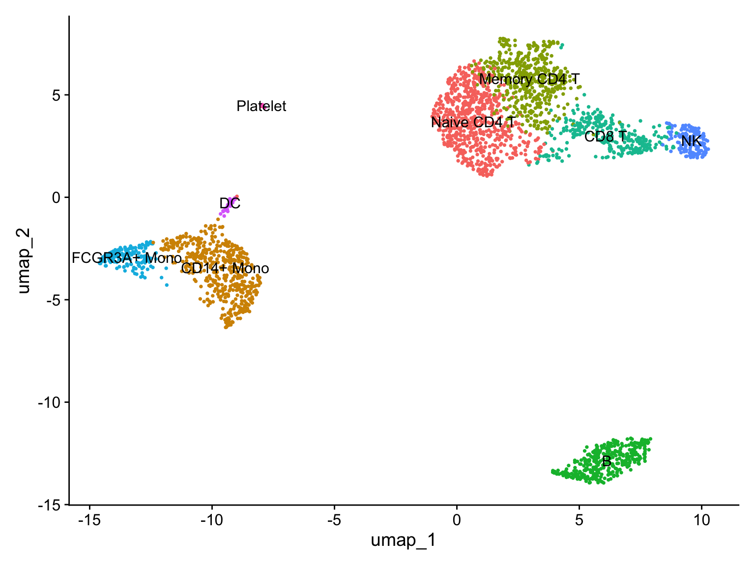
With the mapping decided, RenameIdents() replaces the cluster numbers with cell-type names, in cluster order (0 → 8). The relabelled DimPlot() is the figure the whole analysis was building toward — a map of blood, with every population named.
Modularity Optimizer version 1.3.0 by Ludo Waltman and Nees Jan van Eck

Number of nodes: 2638
Number of edges: 95927

Running Louvain algorithm...
Maximum modularity in 10 random starts: 0.8728
Number of communities: 9
Elapsed time: 0 seconds
pbmc <-RunUMAP(pbmc, dims =1:10)# Map cluster numbers (0-8, in order) to the cell types we read from the markersnew.ids <-c("Naive CD4 T", "CD14+ Mono", "Memory CD4 T", "B", "CD8 T","FCGR3A+ Mono", "NK", "DC", "Platelet")names(new.ids) <-levels(pbmc)pbmc <-RenameIdents(pbmc, new.ids)DimPlot(pbmc, reduction ="umap", label =TRUE, pt.size =0.5) +NoLegend()
Read it as the biology it now encodes. The CD4 T cells (naive and memory) sit together with the CD8 T and NK cells in one connected territory — the lymphocyte continuum, with the cytotoxic populations (CD8 T, NK) at one edge. The two monocyte populations form a second island, with the dendritic cells nearby (all myeloid). The B cells stand apart as their own island, and the platelets — the most distinct population of all — sit completely isolated. The geometry you saw as numbered clusters in C4 is now a labelled map of peripheral blood.
Report it like this. A methods sentence you can paste into a paper:
Cells were clustered on the first 10 principal components (FindNeighbors/FindClusters, resolution 0.5), yielding 9 clusters. Marker genes were identified with FindAllMarkers (Wilcoxon rank-sum test, only.pos = TRUE, min.pct = 0.25, logfc.threshold = 0.25), and clusters were annotated by canonical PBMC markers (IL7R, CCR7, S100A4, CD14, LYZ, MS4A1, CD8A, GZMK, FCGR3A, MS4A7, GNLY, NKG7, FCER1A, CST3, PPBP) as naive CD4 T, memory CD4 T, CD8 T, NK, CD14+ monocytes, FCGR3A+ monocytes, B cells, dendritic cells, and platelets (Seurat 5.4.0).
Common issues
Top markers by fold-change aren’t always the textbook ones. Sorting by avg_log2FC surfaces the most specific genes, which can be obscure (FOLR3, LY6G6F) rather than the famous markers (CD14, PPBP). That is expected — a rare, perfectly cluster-specific gene scores a huge fold-change. Use the unbiased top-markers table to characterize a cluster, but annotate identities from a curated canonical marker panel plotted with FeaturePlot/VlnPlot, where the textbook genes do the naming.
RenameIdents() assigns labels by position, so order matters.names(new.ids) <- levels(pbmc) pairs your labels with the current identities in order (0, 1, 2, …). If your label vector is out of order, you will confidently mislabel every cluster. After renaming, always sanity-check with a DimPlot and a couple of VlnPlots that each named cluster expresses the marker you claim.
A cluster with no clear markers, or two cell types’ markers at once. Sometimes a cluster expresses markers of two lineages (a possible doublet) or has no distinctive genes at all (low-quality cells that slipped past QC). Don’t force a label. Flag it, consider tightening QC or the resolution, and — for doublets specifically — a dedicated tool such as DoubletFinder is the right next step.
Frequently asked questions
NoteHow do I find marker genes for clusters in Seurat?
Run FindAllMarkers(pbmc, only.pos = TRUE, min.pct = 0.25, logfc.threshold = 0.25) on your clustered object. It performs a Wilcoxon rank-sum test for every gene in every cluster (cluster vs all other cells) and returns the up-regulated, well-expressed, clearly-changed genes. Sort each cluster’s markers by avg_log2FC to see its strongest defining genes.
NoteWhat is the difference between FindAllMarkers and FindMarkers?
FindAllMarkers() tests every cluster against all the others in one call — use it to annotate the whole dataset. FindMarkers(ident.1 = "A", ident.2 = "B") compares two specific groups — use it when you want the differentially expressed genes between, say, two T-cell subsets, or one cluster versus one other.
NoteHow do I annotate cell types from marker genes?
Plot a short panel of canonical markers for your tissue (for PBMCs: IL7R, CD14, LYZ, MS4A1, CD8A, FCGR3A, GNLY, NKG7, FCER1A, PPBP) with FeaturePlot() or VlnPlot(), see which cluster each marker lights up, then map cluster → cell type and apply it with RenameIdents(). Always derive the mapping from your own data’s markers — cluster numbers are arbitrary and change with parameters.
NoteWhat do avg_log2FC, pct.1 and pct.2 mean in the marker table?
avg_log2FC is the average log₂ fold-change of the gene in the cluster versus all other cells (higher = stronger marker). pct.1 is the fraction of cells in the cluster expressing the gene; pct.2 is the fraction outside it. A strong marker has a high avg_log2FC and a pct.1 much larger than pct.2.
ImportantYour turn: find a cluster’s markers and check a label
Starting from the clustered pbmc3k object, run FindAllMarkers with the standard settings, pull the top 5 markers for cluster 3 by avg_log2FC, and confirm with a VlnPlot of MS4A1 that cluster 3 is the B cells.
TipHint
Filter the markers data frame to cluster == 3, then slice_max(avg_log2FC, n = 5). VlnPlot(pbmc, features = "MS4A1") shows the per-cluster distribution — the B-cell cluster should be the only one that is high.
TipSolution
library(Seurat)library(dplyr)pbmc.data <-Read10X("_data/filtered_gene_bc_matrices/hg19")pbmc <-CreateSeuratObject(pbmc.data, project ="pbmc3k",min.cells =3, min.features =200)pbmc[["percent.mt"]] <-PercentageFeatureSet(pbmc, pattern ="^MT-")pbmc <-subset(pbmc, subset = nFeature_RNA >200& nFeature_RNA <2500& percent.mt <5)pbmc <-NormalizeData(pbmc)pbmc <-FindVariableFeatures(pbmc, selection.method ="vst", nfeatures =2000)pbmc <-ScaleData(pbmc)pbmc <-RunPCA(pbmc, features =VariableFeatures(pbmc))pbmc <-FindNeighbors(pbmc, dims =1:10)pbmc <-FindClusters(pbmc, resolution =0.5)markers <-FindAllMarkers(pbmc, only.pos =TRUE, min.pct =0.25, logfc.threshold =0.25)markers %>%filter(cluster ==3) %>%slice_max(avg_log2FC, n =5) # LINC00926, VPREB3, CD79A, ... — all B-cell genesVlnPlot(pbmc, features ="MS4A1") # high only in cluster 3
Cluster 3’s top markers include CD79A and MS4A1 — both B-cell genes — and the MS4A1 violin is high in cluster 3 alone. The label “B cells” is well supported.
NoteQuick check: a cluster is high in GNLY and NKG7 but has almost no CD8A. What is it?
A. CD8 T cells — they express cytotoxic genes. B. NK cells — cytotoxic markers without CD8. C. CD14+ monocytes.
TipShow answer
B. NK cells. Both CD8 T cells and NK cells express the cytotoxic genes GNLY and NKG7, so those alone don’t distinguish them. The discriminator is CD8A: present in CD8 T cells, absent in NK cells. High cytotoxic markers withoutCD8A is the NK signature.
Conclusion
Annotation is the payoff of the single-cell workflow, and it is two moves. FindAllMarkers(only.pos = TRUE, min.pct = 0.25, logfc.threshold = 0.25) gives you the genes that define each cluster, and a curated panel of canonical markers — plotted with FeaturePlot and VlnPlot — tells you which known cell type each cluster is. You reasoned from markers to identities (naive vs memory CD4 T from CCR7; CD8 T vs NK from CD8A; classical vs non-classical monocytes from CD14 vs FCGR3A), relabelled with RenameIdents(), and drew the annotated UMAP — a named map of peripheral blood. The durable lesson: cluster numbers are arbitrary, identities come from genes, and an honest annotation says which labels are certain and which are judgment calls.
That completes the pbmc3k guided analysis — from a raw 10x matrix to named cell types. Going further usually means more cells and more conditions: integrating multiple samples, correcting batch effects, scoring cell states, or modelling differentiation trajectories — analyses that are both pipeline-heavy and compute-heavy. That is where a managed compute environment earns its place: the free lessons teach the engine (Seurat), and running it at scale on real datasets is what Arkon is built for.
Ask Prova“how do I find marker genes for my Seurat clusters and annotate them as cell types?” — it answers with R code you can run on your own object, runs FindAllMarkers, plots your canonical markers with FeaturePlot/VlnPlot, and helps you reason from markers to a RenameIdents mapping. The runtime is the judge.Ask Prova →
Was this page helpful?
Thanks for the feedback!
Prove you can do it. Master the whole Single-Cell RNA-Seq Analysis in R series — track your path, build projects, and earn a certificate.
This lesson is reproducible: every figure and number was produced by the code shown — copy any block and run it to reproduce them. The runtime is the judge.
References
Hao, Y., et al. (2021). Integrated analysis of multimodal single-cell data (Seurat v4). Cell, 184(13), 3573–3587.
Satija, R., Farrell, J. A., Gennert, D., Schier, A. F., & Regev, A. (2015). Spatial reconstruction of single-cell gene expression data. Nature Biotechnology, 33(5), 495–502.
Stuart, T., et al. (2019). Comprehensive integration of single-cell data. Cell, 177(7), 1888–1902.
10x Genomics. 3k PBMCs from a Healthy Donor — the canonical pbmc3k filtered gene–barcode matrix (Cell Ranger 1.1.0).