Per-Cell Pathway Activity in R with decoupleR & PROGENy

Go beyond gene-set membership: infer which signaling pathways are firing in each cell from their downstream target genes with PROGENy’s footprint model and decoupleR, validated against a known interferon response

A practical guide to per-cell signaling-pathway activity for single-cell RNA-seq in R. Use the PROGENy footprint model with decoupleR’s multivariate linear model to infer the activity of 14 signaling pathways in every cell, contrast them across an interferon-beta stimulation, and validate the result against the built-in ground truth — IFN-beta signals through JAK-STAT, so JAK-STAT activity must explode in the stimulated cells. Includes how footprint models differ from gene-signature scoring.

TipKey takeaways

• Pathway-activity footprint models ask a different question than gene-set scoring. Signature scoring measures how strongly a cell expresses the genes of a set. A footprint model infers whether a signaling pathway is firing — from the expression of the pathway’s downstream target genes, which move even when the pathway’s own receptor or kinase mRNA looks flat. The footprint is the evidence the pathway leaves behind.
• PROGENy provides the footprint model; decoupleR applies it per cell. PROGENy (Pathway RespOnsive GENes) ships a compendium of 14 signaling pathways, each with a signed set of responsive target genes learned from hundreds of perturbation experiments (Schubert et al., 2018). decoupleR runs that model against every cell’s expression profile to return a per-cell activity score for each pathway (Badia-i-Mompel et al., 2022).
• run_mlm is the recommended engine — a multivariate linear model. It regresses each cell’s expression on all 14 pathways’ target weights at once, so the score for one pathway is adjusted for the others’ overlapping targets. decoupleR also offers run_ulm (univariate), run_wmean and a consensus; run_mlm is the sensible default for PROGENy.
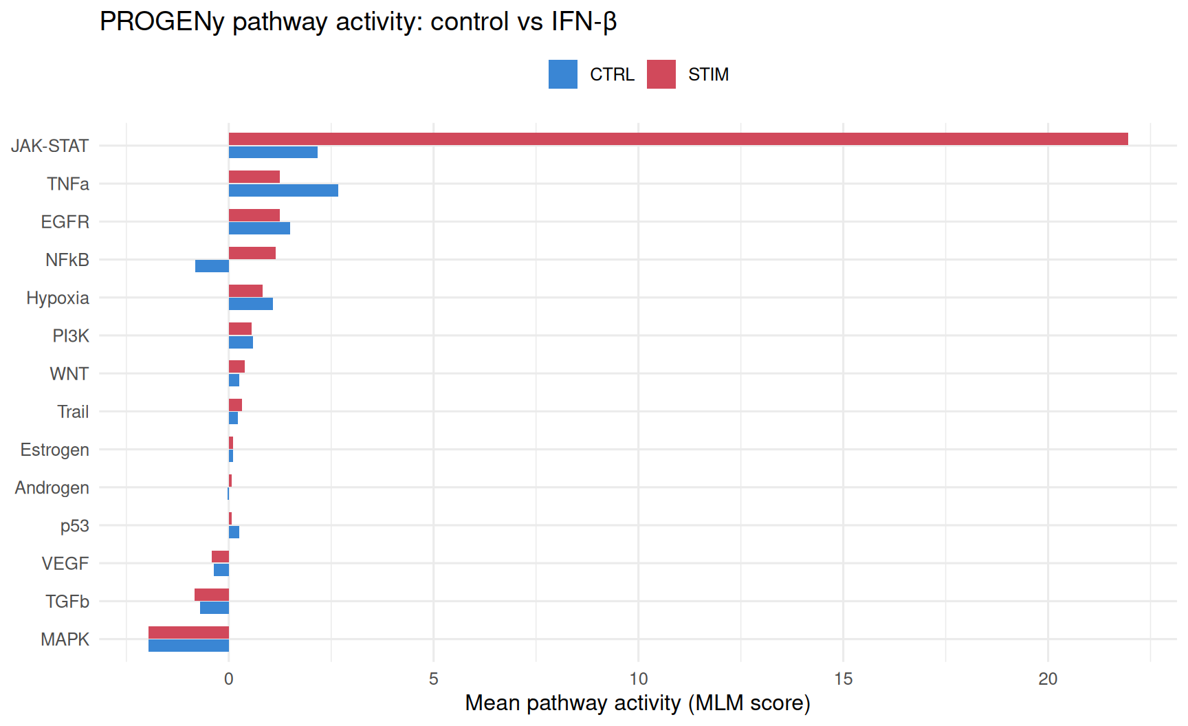
• Validate against a known contrast, at the pathway level. The data has a built-in ground truth: half the cells were stimulated with interferon-beta (IFN-β), which signals through the JAK-STAT pathway. Mean JAK-STAT activity runs 2.2 in the controls and 22.0 in the stimulated cells — a tenfold jump that recovers the biology from target genes alone. NF-κB, the inflammatory pathway, rises too.
• Use footprint models for signaling; use signature scoring for arbitrary programs. Reach for PROGENy + decoupleR when the question is which signaling pathway is active. Reach for per-cell signature scoring when you have a curated gene set — a lineage, a cell state, a custom module — whose membership you want to quantify.

Introduction

You have run the standard single-cell RNA-seq (scRNA-seq) workflow — quality control, clustering, cell-type annotation — and you have started to quantify functional programs per cell. Perhaps you have already scored a few gene signatures. The next question is often sharper: which signaling pathways are actually active in these cells? Not “does this cell express my interferon gene set” but “is the interferon pathway firing?”

That distinction matters because a pathway can be strongly active while its own genes look unremarkable. A receptor is switched on by phosphorylation, not transcription; a kinase cascade runs without any change in the kinase’s mRNA. What does change, reliably, is the set of genes the pathway turns on downstream — its footprint. A footprint model reads that footprint: it infers pathway activity from the expression of the pathway’s transcriptional target genes, the genes that respond when the pathway signals.

This lesson builds per-cell pathway activity with two tools from the Saez-Rodriguez lab: PROGENy (Pathway RespOnsive GENes), which provides the footprint model for 14 signaling pathways, and decoupleR, which applies that model to every cell. We work on the classic IFN-β immune-PBMC benchmark: peripheral blood mononuclear cells (PBMCs — the immune cells in blood) split into a control group and a group stimulated with interferon-beta (IFN-β) (Kang et al., 2018). IFN-β signals through the JAK-STAT pathway, so this design hands us a built-in ground truth: JAK-STAT activity must be far higher in the stimulated cells. If a footprint model cannot recover a signal that strong, we should not trust it on a subtle one.

Footprint models vs signature scoring: two different questions

If you have read the per-cell signature scoring lesson, it is worth being precise about how pathway-activity footprint models differ — because the two are easy to confuse and answer genuinely different questions.

	Gene-signature scoring	Pathway-activity footprint model
Question	How strongly does this cell express this gene set?	Is this signaling pathway firing?
Input genes	The members of the set (the interferon genes themselves)	The pathway’s downstream targets — the genes it regulates
Weights	Usually unweighted membership	Signed weights (a target is induced or repressed)
Catches	Expression of the curated program	Activity even when the pathway’s own genes are flat
Tools	AUCell, UCell, GSVA	PROGENy + decoupleR (this lesson); also for transcription factors
Use when	You have a curated set — a lineage, a state, a module	You want signaling inference — which pathway is on

The key idea: a signature score asks about membership — how enriched a cell is for the genes in the set. A footprint model asks about consequence — whether the transcriptional shadow of an active pathway is visible in the cell. A footprint’s target genes are usually not the pathway’s own components. That is what lets a footprint model report that JAK-STAT is signaling from the induction of interferon-stimulated genes, without ever measuring the activity of the JAK kinases or STAT transcription factors directly.

Both belong in the functional-analysis toolkit; neither replaces the other. The same footprint machinery extends to transcription-factor (TF — a protein that switches genes on or off) activity, where the targets are a TF’s regulated genes.

The data: interferon-stimulated PBMCs with a built-in ground truth

The committed ifnb_subset.rds is a balanced slice of the Kang IFN-β benchmark: a raw count matrix of 13,565 genes across 3,000 cells, plus a metadata table. The stim column records whether each cell was a CTRL (control) or STIM (IFN-β–stimulated) cell — 1,500 of each — and seurat_annotations holds the 13 cell types already called for us. We hold those labels back and use only the stim contrast to validate the pathway activity we infer.

library(Seurat)

d <- readRDS("_data/ifnb_subset.rds")
obj <- CreateSeuratObject(counts = d$counts, meta.data = d$meta)
obj <- NormalizeData(obj, verbose = FALSE)

dim(obj)              # genes x cells

[1] 13565  3000

table(obj$stim)       # the control / IFN-beta contrast: our ground truth

CTRL STIM 
1500 1500 

Log-normalization (NormalizeData) is the one preprocessing step the footprint model assumes: activity is inferred from normalized expression, not raw counts. Every block below rebuilds from exactly this point, so you can copy any one of them and run it on its own.

PROGENy: the footprint model

PROGENy was built by mining a large compendium of perturbation experiments — hundreds of cases where a pathway was deliberately activated or inhibited — and recording which genes consistently responded (Schubert et al., 2018). The result is, for each of 14 signaling pathways, a set of responsive target genes each with a signed weight: a positive weight means the gene goes up when the pathway is active, a negative weight means it goes down. Those weights are the footprint.

The model ships inside the progeny package, so we read it directly — no download. getModel() returns a matrix of genes × pathways, where we keep the top-weighted targets per pathway.

library(progeny)

m <- progeny::getModel(organism = "Human", top = 500)   # top 500 responsive genes per pathway
dim(m)                                                   # genes x 14 pathways

[1] 5782   14

colnames(m)                                              # the 14 signaling pathways

 [1] "Androgen" "EGFR"     "Estrogen" "Hypoxia"  "JAK-STAT" "MAPK"    
 [7] "NFkB"     "p53"      "PI3K"     "TGFb"     "TNFa"     "Trail"   
[13] "VEGF"     "WNT"     

The model covers 5,782 genes across 14 pathways — Androgen, EGFR, Estrogen, Hypoxia, JAK-STAT, MAPK, NFkB, p53, PI3K, TGFb, TNFa, Trail, VEGF and WNT. Each column is one pathway’s signed footprint over those genes.

decoupleR expects the model as a long network table — one row per (pathway, target gene, weight) edge — so we reshape the matrix and drop the zero-weight entries (genes not in a given pathway’s top set).

library(progeny)

m <- progeny::getModel(organism = "Human", top = 500)
net <- data.frame(
  source = rep(colnames(m), each = nrow(m)),   # the pathway
  target = rep(rownames(m), times = ncol(m)),  # the target gene
  weight = as.vector(as.matrix(m)))            # signed footprint weight
net <- net[net$weight != 0, ]                  # keep only real edges

nrow(net)          # 14 pathways x 500 targets = 7000 edges

[1] 7000

head(net)

     source target    weight
8  Androgen  ABCA1 -2.176598
9  Androgen ABCA12 -3.344896
15 Androgen  ABCC1  3.449725
16 Androgen  ABCC4  9.374285
23 Androgen  ABCG1 -2.792402
24 Androgen  ABCG2 -4.016547

That gives 7,000 edges — 500 targets for each of the 14 pathways — the footprint network decoupleR will score.

NoteUse the built-in model, not the network fetch

decoupleR ships a convenience function, get_progeny(), that pulls the same model over the network from the OmnipathR web service. That call needs an internet connection, can hang behind a firewall, and — because the remote resource can change — is not reproducible. Reading the model straight from the packaged progeny::getModel() is offline and deterministic: the numbers on this page are byte-stable across renders. Prefer the packaged model unless you specifically need a newer online version.

decoupleR: infer pathway activity per cell

decoupleR is an ensemble of methods that infer biological activities from omics data within one framework (Badia-i-Mompel et al., 2022). Given an expression matrix and a network of sources (here, pathways) and their weighted targets, it returns an activity score for every source in every cell.

The recommended method for PROGENy is run_mlm — a multivariate linear model (MLM). For each cell it fits one linear regression of the cell’s gene expression on all 14 pathways’ target weights at once; each pathway’s fitted coefficient (its t-value) becomes that pathway’s activity score. Fitting all pathways jointly matters: some target genes belong to more than one pathway, and the multivariate fit adjusts each pathway’s score for the others it shares targets with, rather than crediting the same gene twice.

library(Seurat)
library(decoupleR)
library(progeny)

d <- readRDS("_data/ifnb_subset.rds")
obj <- CreateSeuratObject(counts = d$counts, meta.data = d$meta)
obj <- NormalizeData(obj, verbose = FALSE)
mat <- as.matrix(GetAssayData(obj, layer = "data"))   # genes x cells, normalized

m <- progeny::getModel(organism = "Human", top = 500)
net <- data.frame(source = rep(colnames(m), each = nrow(m)),
                  target = rep(rownames(m), times = ncol(m)),
                  weight = as.vector(as.matrix(m)))
net <- net[net$weight != 0, ]

set.seed(42)
acts <- run_mlm(mat, net, .source = "source", .target = "target",
                .mor = "weight", minsize = 5)
acts <- acts[acts$statistic == "mlm", ]   # keep the MLM score

head(acts)          # long: one row per pathway (source) x cell (condition)

# A tibble: 6 × 5
  statistic source   condition        score p_value
  <chr>     <chr>    <chr>            <dbl>   <dbl>
1 mlm       Androgen AAACATACCAGAAA.1 -1.29 0.198  
2 mlm       EGFR     AAACATACCAGAAA.1  3.27 0.00110
3 mlm       Estrogen AAACATACCAGAAA.1  2.06 0.0397 
4 mlm       Hypoxia  AAACATACCAGAAA.1  2.47 0.0134 
5 mlm       JAK-STAT AAACATACCAGAAA.1 -2.47 0.0133 
6 mlm       MAPK     AAACATACCAGAAA.1 -1.78 0.0752 

The output is a long table: for every cell (the condition column holds the cell barcode) and every pathway (the source column), a score — the pathway’s activity in that cell. The minsize = 5 argument drops any pathway with fewer than five of its targets present in the data, so a score is never built on a handful of genes. From here, the whole analysis is aggregating and plotting that one score.

Validate: JAK-STAT explodes in the stimulated cells

The test of the whole approach is the ground truth. IFN-β signals through JAK-STAT, so JAK-STAT activity must separate the conditions. Average each pathway’s activity within the control and stimulated cells and plot the 14 pathways side by side.

library(Seurat)
library(decoupleR)
library(progeny)
library(ggplot2)

d <- readRDS("_data/ifnb_subset.rds")
obj <- CreateSeuratObject(counts = d$counts, meta.data = d$meta)
obj <- NormalizeData(obj, verbose = FALSE)
mat <- as.matrix(GetAssayData(obj, layer = "data"))
m <- progeny::getModel(organism = "Human", top = 500)
net <- data.frame(source = rep(colnames(m), each = nrow(m)),
                  target = rep(rownames(m), times = ncol(m)),
                  weight = as.vector(as.matrix(m)))
net <- net[net$weight != 0, ]

set.seed(42)
acts <- run_mlm(mat, net, .source = "source", .target = "target",
                .mor = "weight", minsize = 5)
acts <- acts[acts$statistic == "mlm", ]
acts$stim <- obj$stim[match(acts$condition, colnames(obj))]

# Mean activity per pathway per condition (base R aggregation)
agg <- aggregate(score ~ source + stim, data = acts, FUN = mean)
ord <- agg$source[agg$stim == "STIM"][order(agg$score[agg$stim == "STIM"])]
agg$source <- factor(agg$source, levels = ord)

ggplot(agg, aes(x = source, y = score, fill = stim)) +
  geom_col(position = position_dodge(width = 0.7), width = 0.65) +
  coord_flip() +
  scale_fill_manual(values = c(CTRL = "#3a86d4", STIM = "#d1495b")) +
  labs(x = NULL, y = "Mean pathway activity (MLM score)", fill = NULL,
       title = "PROGENy pathway activity: control vs IFN-β") +
  theme_minimal(base_size = 12) +
  theme(legend.position = "top")

The picture is unambiguous. JAK-STAT activity averages 2.2 in the controls and 22.0 in the stimulated cells — a roughly tenfold jump that dwarfs every other pathway. That is the interferon ground truth recovered at the pathway level, and — crucially — recovered from JAK-STAT’s target genes, not from measuring JAK-STAT’s own components. The footprint gives away the signal.

The smaller movers tell a coherent story too. NF-κB, the master inflammatory pathway, rises from -0.8 to 1.2 — interferon stimulation is inflammatory, so an NF-κB increase is exactly right. Meanwhile TNF-α (2.7 → 1.2) and EGFR (1.5 → 1.2) drop. The dominant, unmistakable event is the JAK-STAT explosion, which is the biology the experiment was designed to produce.

See the pathway on the map

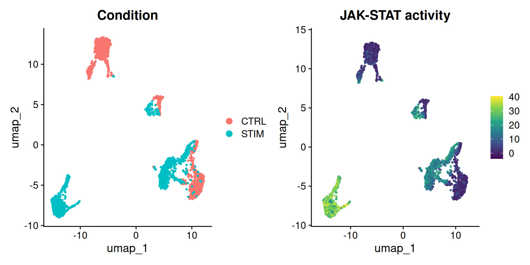
Pathway activity is a per-cell quantity, so it drops straight onto a UMAP (uniform manifold approximation and projection — the 2-D embedding of the cells). Colouring the map by JAK-STAT activity shows the interferon response as a region of the tissue lighting up, tracking the stimulated cells wherever they sit.

set.seed(42)
library(Seurat)
library(decoupleR)
library(progeny)
library(patchwork)
library(ggplot2)

d <- readRDS("_data/ifnb_subset.rds")
obj <- CreateSeuratObject(counts = d$counts, meta.data = d$meta)
obj <- NormalizeData(obj, verbose = FALSE)
mat <- as.matrix(GetAssayData(obj, layer = "data"))
m <- progeny::getModel(organism = "Human", top = 500)
net <- data.frame(source = rep(colnames(m), each = nrow(m)),
                  target = rep(rownames(m), times = ncol(m)),
                  weight = as.vector(as.matrix(m)))
net <- net[net$weight != 0, ]

acts <- run_mlm(mat, net, .source = "source", .target = "target",
                .mor = "weight", minsize = 5)
acts <- acts[acts$statistic == "mlm", ]
js <- acts[acts$source == "JAK-STAT", ]
obj$JAK_STAT <- js$score[match(colnames(obj), js$condition)]

# Standard embedding so the score has a map to land on
obj <- FindVariableFeatures(obj, nfeatures = 2000, verbose = FALSE) |>
  ScaleData(verbose = FALSE) |> RunPCA(npcs = 30, verbose = FALSE) |>
  RunUMAP(dims = 1:30, verbose = FALSE)

p1 <- DimPlot(obj, group.by = "stim") + ggtitle("Condition")
p2 <- FeaturePlot(obj, features = "JAK_STAT") +
  scale_color_viridis_c() + ggtitle("JAK-STAT activity")
p1 + p2

The two panels are almost the same picture: the region the UMAP fills with stimulated cells is exactly the region the JAK-STAT map paints bright. A pathway activity you inferred from downstream targets reproducing the experimental condition you can see in the embedding — that is the visual form of the validation.

Where each pathway is active across cell types

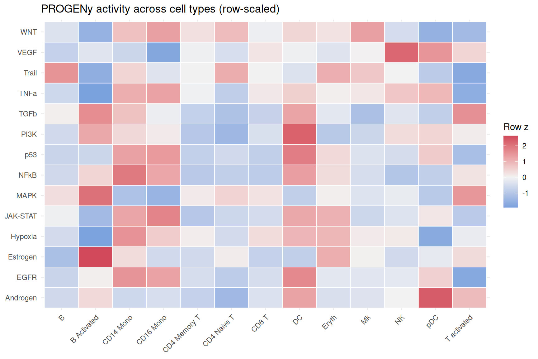
The barplot collapsed each pathway to one number per condition. Activity also varies across cell types, and a heatmap of the 14 pathways over the 13 annotated cell types shows the landscape. To compare cell-type patterns on a common scale despite JAK-STAT’s huge magnitude, we scale each pathway (row) to a z-score across cell types — so each row shows where, relatively, that pathway is most active.

library(Seurat)
library(decoupleR)
library(progeny)
library(ggplot2)

d <- readRDS("_data/ifnb_subset.rds")
obj <- CreateSeuratObject(counts = d$counts, meta.data = d$meta)
obj <- NormalizeData(obj, verbose = FALSE)
mat <- as.matrix(GetAssayData(obj, layer = "data"))
m <- progeny::getModel(organism = "Human", top = 500)
net <- data.frame(source = rep(colnames(m), each = nrow(m)),
                  target = rep(rownames(m), times = ncol(m)),
                  weight = as.vector(as.matrix(m)))
net <- net[net$weight != 0, ]

acts <- run_mlm(mat, net, .source = "source", .target = "target",
                .mor = "weight", minsize = 5)
acts <- acts[acts$statistic == "mlm", ]
acts$ct <- obj$seurat_annotations[match(acts$condition, colnames(obj))]

# Mean activity per pathway per cell type, then z-score each pathway (row)
mn  <- tapply(acts$score, list(acts$source, acts$ct), mean)
z   <- t(scale(t(mn)))    # row-wise z-score across cell types

df <- data.frame(pathway   = rownames(z)[row(z)],
                 cell_type = colnames(z)[col(z)],
                 z         = as.vector(z))
ggplot(df, aes(cell_type, pathway, fill = z)) +
  geom_tile(color = "white", linewidth = 0.3) +
  scale_fill_gradient2(low = "#3a86d4", mid = "grey95", high = "#d1495b",
                       midpoint = 0, name = "Row z") +
  labs(x = NULL, y = NULL, title = "PROGENy activity across cell types (row-scaled)") +
  theme_minimal(base_size = 11) +
  theme(axis.text.x = element_text(angle = 45, hjust = 1))

The interferon signal is not spread evenly. JAK-STAT and NF-κB activity peak in the myeloid compartment — CD14 and CD16 monocytes and dendritic cells — the professional responders that mount the strongest interferon and inflammatory programs. A single condition-level number would have hidden that; the per-cell scores let you see which cells drive the pathway.

Methods, honesty and reproducibility

A few things to keep straight so you use these tools accurately and reproducibly.

run_mlm is one of several decoupleR methods. decoupleR also offers run_ulm (a univariate linear model, fitting each pathway on its own), run_wmean (a weighted mean), run_wsum, and decouple() / run_consensus to combine several. For PROGENy, run_mlm is the documented default because the multivariate fit handles targets shared between pathways; run_ulm is a close, lighter alternative that recovers the same strong JAK-STAT signal but does not adjust pathways for each other. When in doubt, run_mlm is the sensible choice for a weighted footprint model.

The R decoupleR package is now the legacy interface. As of 2025 the Saez-Rodriguez lab has unified development on the Python decoupler 2.0, a faster, more memory-efficient reimplementation that is part of the scverse single-cell ecosystem; the R package is explicitly described as the deprecated version and is in maintenance. The R package still works and is taught here because it plugs straight into a Seurat-based R workflow — but if you are building new pipelines, especially in Python/scanpy, that is the direction of travel. The concepts — footprint models, PROGENy, MLM/ULM inference — are identical across both.

Use the packaged model for reproducible output. As noted above, progeny::getModel() is offline and deterministic, whereas decoupleR’s get_progeny() fetches from the OmnipathR web service (network-dependent, non-reproducible). The results on this page were produced with the packaged model and are byte-stable across renders.

When to use pathway activity vs signature scoring

Both live in the functional-analysis toolkit; choose by the question.

• Reach for PROGENy + decoupleR when the question is signaling — which pathway is active? Footprint models are purpose-built for signaling inference: they read a pathway’s activity from its downstream consequences, catching activity even when the pathway’s own genes are unchanged. The same machinery, with a different network, infers transcription-factor activity (from a TF’s regulated targets).
• Reach for per-cell signature scoring when you have a curated gene set — a lineage signature, a cell-cycle module, an exhaustion program, any list whose membership you want to quantify per cell. AUCell and UCell score how enriched each cell is for the set itself.

In practice they are complementary: score your curated signatures for the programs you have gene lists for, and run a footprint model for the signaling pathways whose activity you want to infer from their targets.

Common issues

get_progeny() hangs or errors about OmnipathR / a network connection. decoupleR::get_progeny() downloads the model from the OmnipathR web service, which needs internet and can stall behind a firewall — and its remote resource can change, so results are not reproducible. Read the model straight from the package instead: progeny::getModel(organism = "Human", top = 500), then build the net data frame as shown. It is offline, deterministic, and identical in structure.

run_mlm warns that too few targets overlap, or a pathway is dropped. The minsize argument (default and here 5) drops any pathway with fewer than that many of its targets present in your matrix. If pathways are disappearing, check that your feature names match the model’s gene symbols (symbols vs Ensembl IDs, species capitalization) — a naming mismatch silently starves the footprint. Lower minsize only if you understand that a score built on very few genes is noisy.

The activity scores are not comparable across pathways. The MLM score is a per-pathway regression statistic, not a normalized quantity on a shared scale — a JAK-STAT score of 22 and an NF-κB score of 1 are not directly comparable in magnitude across pathways. Compare a pathway to itself across conditions or cell types (as the barplot and heatmap do), or z-score within each pathway before comparing rows, rather than reading one pathway’s absolute number against another’s.

Frequently asked questions

NoteWhat is the difference between pathway activity and gene-set (signature) scoring?

Gene-set scoring measures how strongly a cell expresses the genes in a set — its membership. A pathway-activity footprint model infers whether a signaling pathway is firing, from the expression of the pathway’s downstream target genes. The distinction matters because a pathway can be active while its own receptor or kinase genes look flat; its targets betray it. Use footprint models (PROGENy + decoupleR) for signaling inference and signature scoring (AUCell, UCell) for curated gene sets.

NoteWhat is a footprint model?

A footprint model infers the activity of a regulator — a signaling pathway or a transcription factor — from the expression of the genes it regulates, rather than from the regulator’s own expression. The regulated genes are the “footprint” the active regulator leaves in the transcriptome. PROGENy is a footprint model for 14 signaling pathways, built by learning which genes respond consistently across hundreds of perturbation experiments (Schubert et al., 2018).

Noterun_mlm vs run_ulm — which decoupleR method should I use?

run_mlm fits a multivariate linear model, regressing each cell’s expression on all pathways’ target weights at once, so a pathway’s score is adjusted for targets it shares with other pathways. run_ulm fits each pathway univariately, one at a time. For a weighted footprint model like PROGENy, run_mlm is the documented default; run_ulm is a lighter alternative that recovers the same strong signals but does not account for shared targets. decoupleR also offers run_wmean, run_wsum and a consensus over methods.

NoteCan I run decoupleR and PROGENy in Python?

Yes — and for new work it is the actively-developed path. As of 2025 the Saez-Rodriguez lab unified development on the Python decoupler 2.0, part of the scverse ecosystem, which works directly on AnnData/scanpy objects; the R decoupleR is now the legacy interface. The concepts — footprint models, PROGENy, MLM/ULM inference — are identical. This lesson uses the R package because it plugs into a Seurat-based R workflow.

NoteWhy use the packaged PROGENy model instead of decoupleR’s get_progeny()?

decoupleR::get_progeny() fetches the model from the OmnipathR web service over the network, so it needs an internet connection, can hang behind a firewall, and can return different results if the remote resource changes — it is not reproducible. progeny::getModel(organism = "Human", top = 500) reads the same model from the installed package: offline, deterministic, and byte-stable across renders. Prefer the packaged model unless you specifically need a newer online version.

Test your understanding

ImportantYour turn: compare run_mlm with run_ulm on the JAK-STAT contrast

Using ifnb_subset.rds and the PROGENy network, infer pathway activity with run_ulm (the univariate linear model) instead of run_mlm, and compare the JAK-STAT control-vs-stimulated contrast to the run_mlm result in the lesson (2.2 → 22.0). Does the univariate method also recover the interferon ground truth? Compute the mean JAK-STAT activity per condition from run_ulm.

TipHint

run_ulm has the same signature as run_mlm: run_ulm(mat, net, .source = "source", .target = "target", .mor = "weight", minsize = 5). Filter its output to statistic == "ulm", map each cell’s condition (the barcode) to obj$stim, then tapply(score, stim, mean) for the JAK-STAT rows.

TipSolution

library(Seurat); library(decoupleR); library(progeny)
d <- readRDS("_data/ifnb_subset.rds")
obj <- CreateSeuratObject(counts = d$counts, meta.data = d$meta)
obj <- NormalizeData(obj, verbose = FALSE)
mat <- as.matrix(GetAssayData(obj, layer = "data"))
m <- progeny::getModel(organism = "Human", top = 500)
net <- data.frame(source = rep(colnames(m), each = nrow(m)),
                  target = rep(rownames(m), times = ncol(m)),
                  weight = as.vector(as.matrix(m)))
net <- net[net$weight != 0, ]

set.seed(42)
u <- run_ulm(mat, net, .source = "source", .target = "target",
             .mor = "weight", minsize = 5)
u <- u[u$statistic == "ulm", ]
u$stim <- obj$stim[match(u$condition, colnames(obj))]

# JAK-STAT activity by condition, univariate model
js <- u[u$source == "JAK-STAT", ]
tapply(js$score, js$stim, mean)

run_ulm recovers the same ground truth: mean JAK-STAT activity runs about 2.5 in the controls and 22.9 in the stimulated cells — essentially the same tenfold jump run_mlm gave. The strong signal is robust to the method. Where the two differ is on the smaller pathways: because run_ulm scores each pathway independently, it does not down-weight targets shared with other pathways, so pathways like NF-κB read higher than under the multivariate run_mlm. For a clean, dominant signal like interferon the choice barely matters; for teasing apart overlapping pathways, the multivariate run_mlm is the more defensible default.

NoteQuick check: JAK-STAT activity is high in the stimulated cells, but PROGENy’s JAK-STAT footprint contains very few of the classic interferon genes like ISG15 or MX1 themselves. How can the pathway score be high?

A. The score must be wrong — a JAK-STAT footprint should contain the interferon genes. B. A footprint model infers activity from the pathway’s downstream target genes, not the pathway’s own components; those targets respond to JAK-STAT signaling and rise in the stimulated cells, so the inferred activity is high even though the footprint genes differ from the canonical signature. C. The score is high only because the data was not normalized.

TipShow answer

B. That is exactly what a footprint model is designed to do. PROGENy learned, from perturbation experiments, which genes consistently respond when JAK-STAT signals — its footprint. Those responsive targets are not the same as a hand-curated interferon-gene signature; they are the transcriptional consequence of the pathway being active. When IFN-β switches JAK-STAT on, those target genes move, and the model reads the pathway as active — without ever needing the canonical signature genes in the footprint. (Answer A misunderstands footprints; C is wrong — the pipeline normalizes with NormalizeData and the contrast is real.)

Conclusion

Signature scoring asks how strongly a cell expresses a gene set; pathway-activity footprint models ask whether a signaling pathway is firing, inferring it from the pathway’s downstream target genes. PROGENy supplies the footprint model for 14 signaling pathways, and decoupleR’s run_mlm scores it in every cell. On the IFN-β benchmark the method recovered the ground truth cleanly: JAK-STAT activity ran ~10× higher in the stimulated cells — from target genes alone — with NF-κB rising too, and the myeloid cells driving both. Read the pathway to itself across conditions and cell types, validate against a known contrast, and prefer the offline packaged model for reproducible output. Footprint models and signature scoring are complementary entry points to functional single-cell analysis — one for signaling inference, one for curated programs.

Related lessons

• Per-cell gene signature scoring with AUCell & UCell — the membership-based complement to this footprint approach; score a curated gene set per cell and validate it against the same interferon contrast. · Marker genes & cell-type annotation — supplies the cell-type labels the heatmap groups by. · Clustering & UMAP — builds the embedding the pathway scores are painted on. · Pseudobulk differential expression — the condition-level analysis that pairs naturally with pathway activity. · Bioinformatics — the pillar.
• Where this fits: clustering & UMAP → marker genes & annotation → per-cell signature scoring → pathway-activity footprint models with PROGENy & decoupleR → transcription-factor activity in later lessons — from discrete labels to the signaling programs cells run.

🟢 With an AI agent

Ask Prova “how do I infer signaling-pathway activity per cell on my own Seurat object with PROGENy and decoupleR, and validate it against a known contrast?” — it answers with R code you can run on your own data: read the PROGENy model, build the network, call run_mlm(), add the scores to your object, and check them against a condition you already know. The runtime is the judge. Ask Prova →

Was this page helpful?

Prove you can do it. Master the whole Single-Cell RNA-Seq Analysis in R series — track your path, build projects, and earn a certificate.

Start free →

Go Pro — unlimited Prova on your own data and a verifiable certificate that proves the skill.

from $15/mo billed yearly

Go Pro →

✓ You're Pro — keep going. The runtime is the judge.

Get new R & Python lessons by email

Practical, reproducible, no spam. Unsubscribe anytime.

Double opt-in. We never share your email.

Share this pageXLinkedInRedditHN

Note

This lesson is reproducible: every figure and number was produced by the code shown, rendered offline in the datanovia/quarto-bioinformatics Docker image — copy any block and run it to reproduce them. The runtime is the judge.

References

• Schubert, M., Klinger, B., Klünemann, M., Sieber, A., Uhlitz, F., Sauer, S., Garnett, M. J., Blüthgen, N., & Saez-Rodriguez, J. (2018). Perturbation-response genes reveal signaling footprints in cancer gene expression — introduces PROGENy. Nature Communications, 9, 20. https://doi.org/10.1038/s41467-017-02391-6
• Badia-i-Mompel, P., Vélez Santiago, J., Braunger, J., Geiss, C., Dimitrov, D., Müller-Dott, S., Taus, P., Dugourd, A., Holland, C. H., Ramirez Flores, R. O., & Saez-Rodriguez, J. (2022). decoupleR: ensemble of computational methods to infer biological activities from omics data. Bioinformatics Advances, 2(1), vbac016. https://doi.org/10.1093/bioadv/vbac016
• Kang, H. M., et al. (2018). Multiplexed droplet single-cell RNA-sequencing using natural genetic variation — the source of the IFN-β–stimulated PBMC dataset. Nature Biotechnology, 36, 89–94. https://doi.org/10.1038/nbt.4042
• decoupler (Python, actively developed) — scverse. https://github.com/scverse/decoupler · decoupleR (R, legacy) — Saez-Rodriguez lab. https://github.com/saezlab/decoupleR