Barplot (also known as Bar Graph or Column Graph) is used to show discrete, numerical comparisons across categories. One axis of the chart shows the specific categories being compared and the other axis represents a discrete value scale.
This article describes how to create a barplot using the ggplot2 R package.
You will learn how to:
- Create basic and grouped barplots
- Add labels to a barplot
- Change the bar line and fill colors by group
Contents:
Related Book
GGPlot2 Essentials for Great Data Visualization in RKey R functions
- Key function:
geom_col()for creating bar plots. The heights of the bars represent values in the data. - Key arguments to customize the plot:
color,fill: bar border and fill colorwidth: bar width
Data preparation
We’ll create two data frames derived from the ToothGrowth datasets.
df <- data.frame(dose=c("D0.5", "D1", "D2"),
                len=c(4.2, 10, 29.5))

head(df)
## dose len
## 1 D0.5 4.2
## 2 D1 10.0
## 3 D2 29.5df2 <- data.frame(supp=rep(c("VC", "OJ"), each=3),
dose=rep(c("D0.5", "D1", "D2"),2),
len=c(6.8, 15, 33, 4.2, 10, 29.5))
head(df2)## supp dose len
## 1 VC D0.5 6.8
## 2 VC D1 15.0
## 3 VC D2 33.0
## 4 OJ D0.5 4.2
## 5 OJ D1 10.0
## 6 OJ D2 29.5len: Tooth lengthdose: Dose in milligrams (0.5, 1, 2)supp: Supplement type (VC or OJ)
Loading required R package
Load the ggplot2 package and set the default theme to theme_classic() with the legend at the top of the plot:
library(ggplot2)
theme_set(
  theme_classic() +
    theme(legend.position = "top")
  )
Basic barplots
We start by creating a simple barplot (named f) using the df data set:
f <- ggplot(df, aes(x = dose, y = len))# Basic bar plot
f + geom_col()
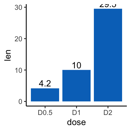
# Change fill color and add labels at the top (vjust = -0.3)
f + geom_col(fill = "#0073C2FF") +
geom_text(aes(label = len), vjust = -0.3)
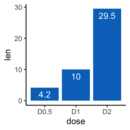
# Label inside bars, vjust = 1.6
f + geom_col(fill = "#0073C2FF")+
geom_text(aes(label = len), vjust = 1.6, color = "white")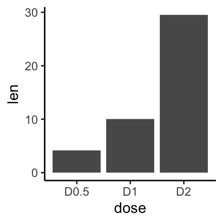
Note that, it’s possible to change the width of bars using the argument width (e.g.: width = 0.5)
Change barplot colors by groups
We’ll change the barplot line and fill color by the variable dose group levels. To set a palette of custom color the function scale_color_manual() is used.
# Change barplot line colors by groups
f + geom_col(aes(color = dose), fill = "white") +
scale_color_manual(values = c("#00AFBB", "#E7B800", "#FC4E07"))
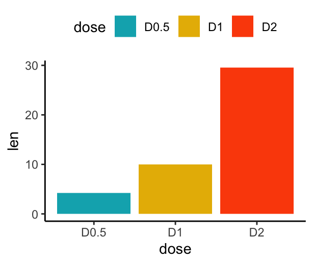
# Change barplot fill colors by groups
f + geom_col(aes(fill = dose)) +
scale_fill_manual(values = c("#00AFBB", "#E7B800", "#FC4E07"))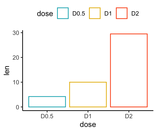
Barplot with multiple groups
Create stacked and dodged bar plots. Use the functions scale_color_manual() and scale_fill_manual() to set manually the bars border line colors and area fill colors.
# Stacked bar plots of y = counts by x = cut,
# colored by the variable color
ggplot(df2, aes(x = dose, y = len)) +
geom_col(aes(color = supp, fill = supp), position = position_stack()) +
scale_color_manual(values = c("#0073C2FF", "#EFC000FF"))+
scale_fill_manual(values = c("#0073C2FF", "#EFC000FF"))
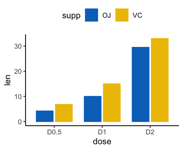
# Use position = position_dodge()
p <- ggplot(df2, aes(x = dose, y = len)) +
geom_col(aes(color = supp, fill = supp), position = position_dodge(0.8), width = 0.7) +
scale_color_manual(values = c("#0073C2FF", "#EFC000FF"))+
scale_fill_manual(values = c("#0073C2FF", "#EFC000FF"))
p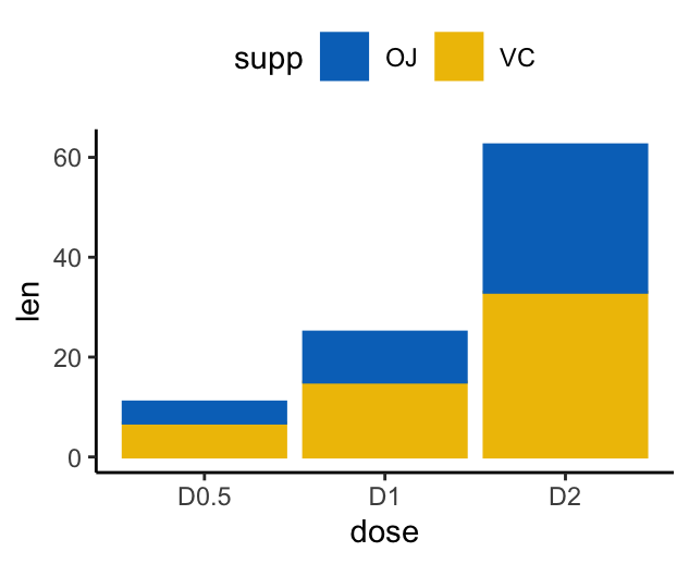
Note that, position_stack() automatically stack values in reverse order of the group aesthetic. This default ensures that bar colors align with the default legend. You can change this behavior by using position = position_stack(reverse = TRUE).
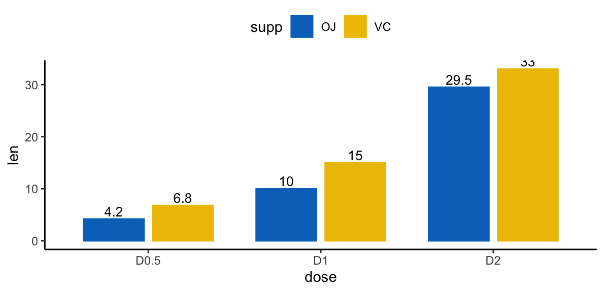
Add labels to a dodged barplot:
p + geom_text(
  aes(label = len, group = supp),
  position = position_dodge(0.8),
  vjust = -0.3, size = 3.5
)
Add labels to a stacked bar plots. 4 steps required to compute the position of text labels:
- Group the data by the dose variable
- Sort the data by
doseandsuppcolumns. Asposition_stack()reverse the group order,suppcolumn should be sorted in descending order. - Calculate the cumulative sum of
lenfor eachdosecategory. Used as the y coordinates of labels. To put the label in the middle of the bars, we’ll usecumsum(len) - 0.5 * len. - Create the bar graph and add labels
# Arrange/sort and compute cumulative summs
library(dplyr)
 df2 <- df2 %>%
  group_by(dose) %>%
  arrange(dose, desc(supp)) %>%
  mutate(lab_ypos = cumsum(len) - 0.5 * len)
df2
## # A tibble: 6 x 4
## # Groups: dose [3]
## supp dose len lab_ypos
## <fct> <fct> <dbl> <dbl>
## 1 VC D0.5 6.8 3.4
## 2 OJ D0.5 4.2 8.9
## 3 VC D1 15 7.5
## 4 OJ D1 10 20
## 5 VC D2 33 16.5
## 6 OJ D2 29.5 47.8# Create stacked bar graphs with labels
ggplot(data = df2, aes(x = dose, y = len)) +
geom_col(aes(fill = supp), width = 0.7)+
geom_text(aes(y = lab_ypos, label = len, group =supp), color = "white") +
scale_color_manual(values = c("#0073C2FF", "#EFC000FF"))+
scale_fill_manual(values = c("#0073C2FF", "#EFC000FF"))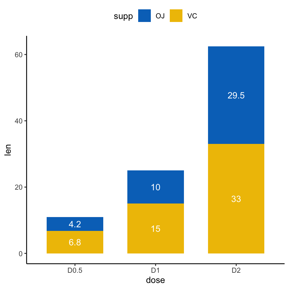
Conclusion
This article describes how to create and customize barplot using the ggplot2 R package.
Recommended for you
This section contains best data science and self-development resources to help you on your path.
Books - Data Science
Our Books
- Practical Guide to Cluster Analysis in R by A. Kassambara (Datanovia)
- Practical Guide To Principal Component Methods in R by A. Kassambara (Datanovia)
- Machine Learning Essentials: Practical Guide in R by A. Kassambara (Datanovia)
- R Graphics Essentials for Great Data Visualization by A. Kassambara (Datanovia)
- GGPlot2 Essentials for Great Data Visualization in R by A. Kassambara (Datanovia)
- Network Analysis and Visualization in R by A. Kassambara (Datanovia)
- Practical Statistics in R for Comparing Groups: Numerical Variables by A. Kassambara (Datanovia)
- Inter-Rater Reliability Essentials: Practical Guide in R by A. Kassambara (Datanovia)
Others
- R for Data Science: Import, Tidy, Transform, Visualize, and Model Data by Hadley Wickham & Garrett Grolemund
- Hands-On Machine Learning with Scikit-Learn, Keras, and TensorFlow: Concepts, Tools, and Techniques to Build Intelligent Systems by Aurelien Géron
- Practical Statistics for Data Scientists: 50 Essential Concepts by Peter Bruce & Andrew Bruce
- Hands-On Programming with R: Write Your Own Functions And Simulations by Garrett Grolemund & Hadley Wickham
- An Introduction to Statistical Learning: with Applications in R by Gareth James et al.
- Deep Learning with R by François Chollet & J.J. Allaire
- Deep Learning with Python by François Chollet
Version:
 Français

No Comments