Data Visualization using GGPlot2

Data Visualization using GGPlot2
Featured

Data Visualization using GGPlot2

Course description

Data visualization is an important component for data science.

This course presents the essentials of ggplot2 to easily create beautiful graphics in R. GGPlot2 is a powerful and popular R package for producing professional graphics piece by piece.

At the end of this course, you will be familiar with ggplot2 concepts that will allow you to efficiently create complex graphics. You will also learn how to combine multiple ggplots into one figure.

Related Book

GGPlot2 Essentials for Great Data Visualization in R

Key features of this course

Some key features of this course include:

  • Covers the most important graphic functions
  • Short, self-contained chapters with practical examples.

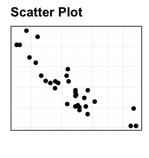
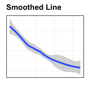
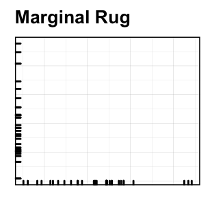
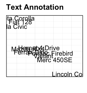
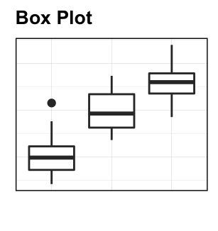
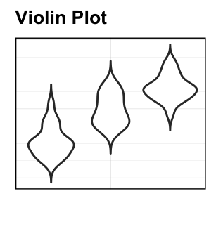
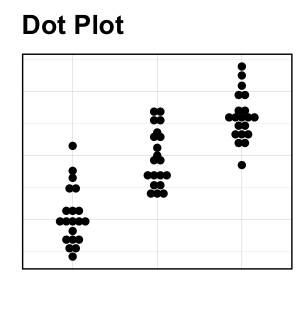
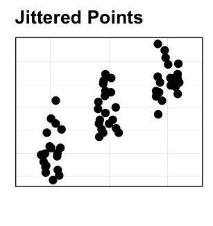
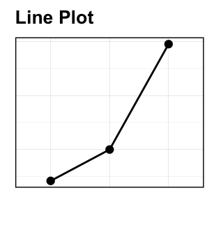
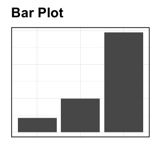
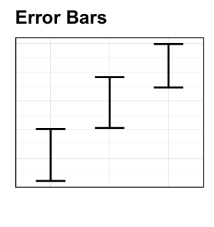
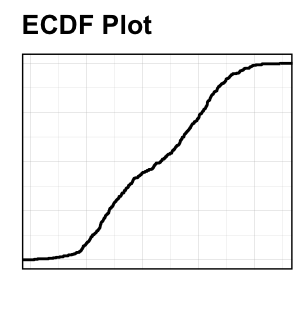
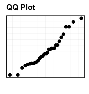
Some examples of graphs, described in this course, are shown below.

  • Create Scatter plots to display the relationship between two continuous variables x and y

  • Using Box plots and alternatives to visualize data grouped by the levels of a categorical variable

  • Bar and Line Plots

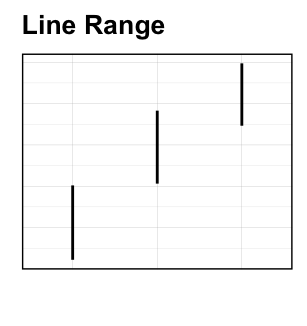
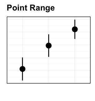
  • Visualizing error bars

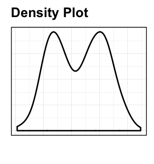
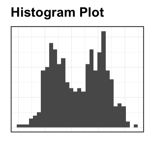
  • Inspecting the distribution of a continuous variable using density plots, histograms and alternatives

Installing Required R packages

Install the following R packages:

  • tidyverse packages for easy data manipulation and visualization.
  • ggpubr package, which makes it easy, for beginner, to create publication ready plots.
install.packages("tidyverse")
install.packages("ggpubr")

Demo datasets

We’ll mainly used the following demo datasets available in R:

  • iris, which gives the measurements in centimeters of the variables sepal length and width and petal length and width, respectively, for 50 flowers from each of 3 species of iris. The species are Iris setosa, versicolor, and virginica.
  • ToothGrowth, which gives the effect of Vitamin C on tooth growth in guinea pigs

To learn more about these datasets, type this in R console:

?iris

?ToothGrowth


Version: Français

Lessons

  1. This article presents the basics of ggplot2. The key ggplot graphic functions are presented. You will learn how to build a ggplot piece by piece, as well as, how to customize and export the plot
  2. A Scatter plot is used to display the relationship between two continuous variables x and y. This article describes how to create scatter plots in R using the ggplot2 package. You will learn how to: 1) Color points by groups; 2) Create bubble charts; 3) Add regression line to a scatter plot.
  3. Boxplots are used to visualize the distribution of a grouped continuous variable through their quartiles. You will learn how to create and customize boxplots using the ggplot2 R package.
  4. A Violin Plot is used to visualize the distribution of the data and its probability density. This chart is a combination of a Box plot and a Density Plot that is rotated and placed on each side, to display the distribution shape of the data. A Violin Plot shows more information than a Box Plot. For example, in a violin plot, you can see whether the distribution of the data is bimodal or multimodal. This article describes how to create and customize violin plots using the ggplot2 R package.
  5. A Dot Plot is used to visualize the distribution of the data. This chart creates stacked dots, where each dot represents one observation. Summary statistics are usually added to dotplots for indicating, for example, the median of the data and the interquartile range. This article describes how to create and customize Dot Plots using the ggplot2 R package.
  6. Stripcharts are also known as one dimensional scatter plots. These plots are suitable compared to box plots when sample sizes are small. This article describes how to create and customize Stripcharts using the ggplot2 R package.
  7. In a line plot, observations are ordered by x value and connected by a line. This article describes how to create a line plot using the ggplot2 R package. You will learn how to: 1) Create basic and grouped line plots; 2) Add points to a line plot; 3) Change the line types and colors by group.
  8. Barplot is used to show discrete, numerical comparisons across categories. One axis of the chart shows the specific categories being compared and the other axis represents a discrete value scale.This article describes how to create a barplot using the ggplot2 R package.You will learn how to: 1) Create basic and grouped barplots; 2) Add labels to a barplot; 3) Change the bar line and fill colors by group
  9. Error Bars are used to visualize the variability of the plotted data. Error Bars can be applied to graphs such as, Dot Plots, Barplots or Line Graphs, to provide an additional layer of detail on the presented data. Generally, Error bars are used to show either the standard deviation, standard error, confidence intervals or interquartile range. The length of an Error Bar helps reveal the uncertainty of a data point. This article describes how to add error bars into a plot using the ggplot2 R package. You will learn how to create bar plots and line plots with error bars
  10. A density plot is an alternative to Histogram used for visualizing the distribution of a continuous variable. The peaks of a Density Plot help to identify where values are concentrated over the interval of the continuous variable. Compared to Histograms, Density Plots are better at finding the distribution shape because they are re not affected by the number of bins used (each bar used in a typical histogram). This article describes how to create density plots using the ggplot2 R package.
  11. A histogram plot is an alternative to Density plot for visualizing the distribution of a continuous variable. This chart represents the distribution of a continuous variable by dividing into bins and counting the number of observations in each bin. This article describes how to create Histogram plots using the ggplot2 R package.
  12. A Quantile-quantile plot (or QQPlot) is used to check whether a given data follows normal distribution. The data is assumed to be normally distributed when the points approximately follow the 45-degree reference (diagonal) line. This article describes how to create a qqplot in R using the ggplot2 package.
  13. ECDF (or Empirical cumulative distribution function) provides an alternative visualization of distribution. It reports for any given number the percent of individuals that are below that threshold. This article describes how to create an ECDF in R using the function stat_ecdf() in ggplot2 package.
  14. This article describes how to combine multiple ggplots into a figure. You will learn how to use: 1) ggplot2 facet functions for creating multiple panel figures that share the same axes; 2) ggarrange() functiong [ggpubr package] for combining independent ggplots.

Comments ( 3 )

  • Limbu M. Limbu

    Do these courses have videos?

    • Kassambara

      These courses are only text courses

  • H

    Do we get a certificate from the course?

Give a comment

Want to post an issue with R? If yes, please make sure you have read this: How to Include Reproducible R Script Examples in Datanovia Comments

Teachers