Friedman Test in R: Non-Parametric Repeated-Measures Comparison

Compare three or more paired (repeated) groups without the normality assumption — the Friedman test the modern way, with Kendall’s W effect size and pairwise follow-ups

Learn to run the Friedman test in R with rstatix — the non-parametric alternative to the one-way repeated-measures ANOVA, for three or more paired groups when normality fails or the outcome is ordinal. Compute the test, the Kendall’s W effect size, and pairwise Wilcoxon signed-rank comparisons, then put the p-values on the plot.

TipKey takeaways

• The Friedman test is the non-parametric alternative to the one-way repeated-measures ANOVA: it compares three or more paired groups (the same subjects measured repeatedly) without assuming normality.
• Use it when the repeated-measures ANOVA normality assumption fails, or the outcome is ordinal.
• Run it with rstatix friedman_test(score ~ time | id) — | id identifies the repeated subject.
• Report the Kendall’s W effect size (friedman_effsize()): 0.1 small, 0.3 moderate, ≥ 0.5 large.
• Follow a significant result with pairwise Wilcoxon signed-rank tests (Bonferroni-adjusted) to see which time points differ.

Introduction

The Friedman test assesses whether three or more paired groups differ — the same participants measured under several conditions or over time. It is the non-parametric counterpart of the one-way repeated-measures ANOVA, and it extends the sign test from two paired groups to many. Because it works on ranks, it makes no normality assumption and handles ordinal outcomes.

Reach for it when the repeated-measures ANOVA assumptions don’t hold — non-normal differences, small samples, or rating-scale data. The scenario here: self-esteem measured at three time points on the same people — do the scores differ across time? This lesson runs the workflow with rstatix on the selfesteem dataset.

Note

Friedman test hypotheses. H₀: the distributions of the repeated groups are the same (no difference across conditions). Hₐ: at least one group’s distribution differs. The test ranks each subject’s values across conditions and compares the rank totals.

The data: self-esteem over three time points

We use the selfesteem dataset from datarium — self-esteem score for 10 people at three times (t1/t2/t3). The Friedman test needs long format, built with base R:

library(rstatix)

data("selfesteem", package = "datarium")
n <- nrow(selfesteem)
long <- data.frame(
  id    = factor(rep(selfesteem$id, 3)),
  time  = factor(rep(c("t1", "t2", "t3"), each = n)),
  score = c(selfesteem$t1, selfesteem$t2, selfesteem$t3)
)
head(long, 3)

  id time    score
1  1   t1 4.005027
2  2   t1 2.558124
3  3   t1 3.244241

Summarize the score at each time point:

library(rstatix)

data("selfesteem", package = "datarium")
n <- nrow(selfesteem)
long <- data.frame(
  id = factor(rep(selfesteem$id, 3)), time = factor(rep(c("t1", "t2", "t3"), each = n)),
  score = c(selfesteem$t1, selfesteem$t2, selfesteem$t3)
)

long %>%
  group_by(time) %>%
  get_summary_stats(score, type = "common")

# A tibble: 3 × 11
  time  variable     n   min   max median   iqr  mean    sd    se    ci
  <fct> <fct>    <dbl> <dbl> <dbl>  <dbl> <dbl> <dbl> <dbl> <dbl> <dbl>
1 t1    score       10  2.05  4.00   3.21 0.571  3.14 0.552 0.174 0.395
2 t2    score       10  3.91  6.91   4.60 0.89   4.93 0.863 0.273 0.617
3 t3    score       10  6.31  9.78   7.46 1.74   7.64 1.14  0.361 0.817

Look at the data first

A boxplot with the individual points shows each subject’s trajectory across time:

library(rstatix)
library(ggpubr)

data("selfesteem", package = "datarium")
n <- nrow(selfesteem)
long <- data.frame(
  id = factor(rep(selfesteem$id, 3)), time = factor(rep(c("t1", "t2", "t3"), each = n)),
  score = c(selfesteem$t1, selfesteem$t2, selfesteem$t3)
)

ggboxplot(long, x = "time", y = "score", add = "jitter", color = "#3a86d4")

Run the Friedman test

friedman_test() takes a score ~ time | id formula — the outcome by the repeated factor, with | id naming the subject identifier:

library(rstatix)

data("selfesteem", package = "datarium")
n <- nrow(selfesteem)
long <- data.frame(
  id = factor(rep(selfesteem$id, 3)), time = factor(rep(c("t1", "t2", "t3"), each = n)),
  score = c(selfesteem$t1, selfesteem$t2, selfesteem$t3)
)

res.fried <- long %>% friedman_test(score ~ time | id)
res.fried

# A tibble: 1 × 6
  .y.       n statistic    df        p method       
* <chr> <int>     <dbl> <dbl>    <dbl> <chr>        
1 score    10      18.2     2 0.000112 Friedman test

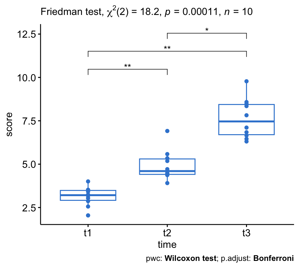
Self-esteem differs significantly across the three time points, χ²(2) = 18.2, p = 0.0001 — at least one time point’s distribution is different.

Effect size: Kendall’s W

The Kendall’s W coefficient measures how large the effect is, from 0 (no agreement) to 1 (perfect):

library(rstatix)

data("selfesteem", package = "datarium")
n <- nrow(selfesteem)
long <- data.frame(
  id = factor(rep(selfesteem$id, 3)), time = factor(rep(c("t1", "t2", "t3"), each = n)),
  score = c(selfesteem$t1, selfesteem$t2, selfesteem$t3)
)

long %>% friedman_effsize(score ~ time | id)

# A tibble: 1 × 5
  .y.       n effsize method    magnitude
* <chr> <int>   <dbl> <chr>     <ord>    
1 score    10    0.91 Kendall W large    

W = 0.91 is a large effect (the benchmarks are 0.1 small, 0.3 moderate, ≥ 0.5 large) — time has a strong influence on self-esteem.

Post-hoc: which time points differ?

A significant Friedman test is followed up with pairwise Wilcoxon signed-rank tests (the paired, non-parametric comparison), Bonferroni-adjusted:

library(rstatix)

data("selfesteem", package = "datarium")
n <- nrow(selfesteem)
long <- data.frame(
  id = factor(rep(selfesteem$id, 3)), time = factor(rep(c("t1", "t2", "t3"), each = n)),
  score = c(selfesteem$t1, selfesteem$t2, selfesteem$t3)
)

pwc <- long %>%
  wilcox_test(score ~ time, paired = TRUE, p.adjust.method = "bonferroni")
pwc

# A tibble: 3 × 9
  .y.   group1 group2    n1    n2 statistic     p p.adj p.adj.signif
* <chr> <chr>  <chr>  <int> <int>     <dbl> <dbl> <dbl> <chr>       
1 score t1     t2        10    10         0 0.002 0.006 **          
2 score t1     t3        10    10         0 0.002 0.006 **          
3 score t2     t3        10    10         1 0.004 0.012 *           

All three pairwise differences are significant: t1–t2 (p.adj = 0.006), t1–t3 (p.adj = 0.006) and t2–t3 (p.adj = 0.012) — self-esteem rises significantly at each step.

Plot it with the p-values

library(rstatix)
library(ggpubr)

data("selfesteem", package = "datarium")
n <- nrow(selfesteem)
long <- data.frame(
  id = factor(rep(selfesteem$id, 3)), time = factor(rep(c("t1", "t2", "t3"), each = n)),
  score = c(selfesteem$t1, selfesteem$t2, selfesteem$t3)
)

res.fried <- long %>% friedman_test(score ~ time | id)
pwc <- long %>%
  wilcox_test(score ~ time, paired = TRUE, p.adjust.method = "bonferroni") %>%
  add_xy_position(x = "time")

ggboxplot(long, x = "time", y = "score", add = "point", color = "#3a86d4") +
  stat_pvalue_manual(pwc, hide.ns = TRUE) +
  labs(
    subtitle = get_test_label(res.fried, detailed = TRUE),
    caption = get_pwc_label(pwc)
  )

Report

The self-esteem score differed significantly across the three time points, as assessed by a Friedman test, χ²(2) = 18.2, p = 0.0001, with a large effect size (Kendall’s W = 0.91). Pairwise Wilcoxon signed-rank tests (Bonferroni-adjusted) showed significant increases between t1 and t2 (p = 0.006), t1 and t3 (p = 0.006), and t2 and t3 (p = 0.012).

NoteThe math (optional)

The Friedman test ranks each subject’s values across the \(k\) conditions (so ranks run 1…\(k\) within each row), sums the ranks per condition, and compares those rank totals to what equal distributions would give. The statistic \(\chi^2_F = \frac{12}{N k (k+1)} \sum_j R_j^2 - 3N(k+1)\) (with \(R_j\) the rank total for condition \(j\), \(N\) subjects, \(k\) conditions) follows a chi-square distribution with \(k-1\) degrees of freedom. Kendall’s \(W = \chi^2_F / [N(k-1)]\) rescales it to a 0–1 effect size.

Try it live

Run the Friedman workflow on a different repeated-measures question, or edit the post-hoc step. The sandbox boots on first Run.

🟢 With an AI agent

Ask Prova “I have the same subjects measured at three or more time points and my data isn’t normal — run a Friedman test on my data, give the Kendall’s W effect size, and tell me which time points differ” — it answers with rstatix code you can run on your own data. The runtime is the judge. Ask Prova →

Common issues

Your data is in wide format. friedman_test() needs long format — one row per measurement with id, the repeated factor and the score. Reshape the wide columns first.

You used a regular Wilcoxon (not paired) for the post-hoc. The follow-up must be the paired Wilcoxon signed-rank test (paired = TRUE) because the groups are repeated measures of the same subjects — and the data must be ordered consistently by id so the pairs line up.

You ran a repeated-measures ANOVA despite non-normal data. If the within-subject differences are clearly non-normal or the outcome is ordinal, the Friedman test is the correct choice — the ANOVA’s F-statistic is not trustworthy there.

Frequently asked questions

NoteWhat is the Friedman test used for?

The Friedman test compares three or more paired (repeated) groups — the same subjects measured under several conditions or over time — to see whether their distributions differ. It is the non-parametric alternative to the one-way repeated-measures ANOVA, used when normality fails or the outcome is ordinal.

NoteWhat is the difference between the Friedman test and repeated-measures ANOVA?

Both compare three or more paired groups, but the repeated-measures ANOVA is parametric (assumes normally distributed differences and tests means), while the Friedman test is non-parametric (works on ranks, no normality assumption). Use Friedman when the ANOVA assumptions are violated or the data are ordinal.

NoteWhat post-hoc test follows a significant Friedman test?

Pairwise Wilcoxon signed-rank tests (the paired, non-parametric comparison), with a multiple-testing correction such as Bonferroni. This identifies which specific pairs of conditions differ after the overall Friedman test is significant.

NoteWhat effect size should I report for the Friedman test?

Kendall’s W (friedman_effsize()), which ranges from 0 (no effect) to 1 (perfect), interpreted with Cohen’s benchmarks: 0.1 small, 0.3 moderate, ≥ 0.5 large. Report it alongside the chi-square statistic and p-value.

Test your understanding

ImportantPractice

1. Run it. In the live cell, run the Friedman test of score by time with subject id. Fill the blank in the formula. Is the result significant, and what is Kendall’s W?
2. Conceptual. Your repeated-measures data fails the normality assumption. Why is the Friedman test the right choice, and what post-hoc test would you use?

NoteHint

Complete the formula as score ~ time | id — time is the repeated factor and id the subject. The output gives the chi-square statistic and p-value; add friedman_effsize() for Kendall’s W. For question 2, recall what assumption the Friedman test doesn’t make.

NoteSolution

long |> friedman_test(score ~ time | id)
#> chi-square(2) = 18.2, p = 0.0001 — significant.
long |> friedman_effsize(score ~ time | id)
#> Kendall's W = 0.91 (large).

The test is significant with a large effect. For question 2: the Friedman test is non-parametric, so it makes no normality assumption — the right choice when the within-subject differences aren’t normal. Follow it with pairwise Wilcoxon signed-rank tests.

TipWhich test when?

• Three or more paired groups, normal → repeated-measures ANOVA.
• Three or more paired groups, non-normal / ordinal → Friedman test (this lesson).
• Three or more independent groups, non-normal → Kruskal-Wallis test.
• Two paired groups, non-normal → Wilcoxon signed-rank or the sign test.

Conclusion

You can now run the Friedman test in R: reshape to long format, run friedman_test(score ~ time | id), report Kendall’s W for the effect size, and follow a significant result with pairwise Wilcoxon signed-rank tests to locate the differences. It is the test to reach for whenever you have three or more repeated measurements and the repeated-measures ANOVA’s normality assumption doesn’t hold.

Related lessons

• Repeated-measures ANOVA in R — the parametric version, when normality holds. · Kruskal-Wallis test in R — the non-parametric test for independent groups. · Sign test in R — the two-paired-group non-parametric test Friedman generalises. · Normality test in R — the check that decides parametric vs non-parametric.
• Go further: The ANOVA family · Biostatistics

Was this page helpful?

Prove you can do it. Master the whole ANOVA in R series — track your path, build projects, and earn a certificate.

Start free →

Go Pro — unlimited Prova on your own data and a verifiable certificate that proves the skill.

from $15/mo billed yearly

Go Pro →

✓ You're Pro — keep going. The runtime is the judge.

Ready to level up?

Prove it — earn the ANOVA & Multi-Group Comparisons certificate.Take the assessment →Try this on your own data with Prova — the runtime is the judge.Open Prova →

Get new R & Python lessons by email

Practical, reproducible, no spam. Unsubscribe anytime.

Double opt-in. We never share your email.

Share this pageXLinkedInRedditHN

Note

Every result on this page was produced by the code shown, run at build time against a pinned R environment — edit any block and Run to reproduce it yourself.