Log-Rank Test in R: Compare Survival Curves Between Groups

Test whether survival differs between groups with survdiff() — read the chi-square and p-value, then draw a Kaplan-Meier curve with the log-rank p on the plot

Learn the log-rank test in R with the survival and survminer packages. Compare survival between groups on the NCCTG lung-cancer data with survdiff(), read the chi-square statistic, degrees of freedom, and p-value in plain language, and draw the signature Kaplan-Meier plot with the log-rank p-value, risk table, and confidence bands on it.

TipKey takeaways

• The log-rank test (survdiff()) is the standard test for asking “does survival differ between groups?” — treatment vs control, male vs female, by disease stage. It compares the whole survival curves, not survival at a single time point.
• It is non-parametric: it makes no assumption about the shape of the survival distributions. It works on the observed vs expected number of events in each group and returns a chi-square statistic and a p-value.
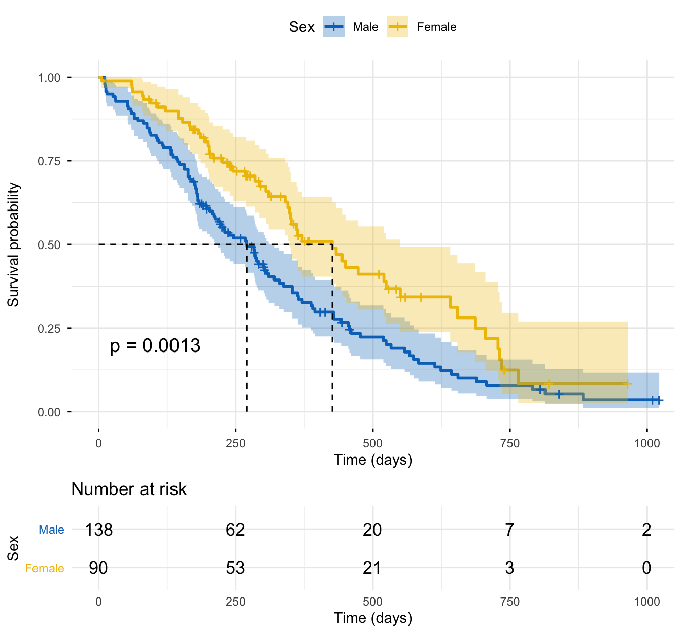
• On the lung-cancer data, survival differs significantly between the sexes: χ² = 10.3, df = 1, p = 0.0013 — females live longer (median 426 vs 270 days).
• Run it with survdiff(Surv(time, status) ~ group, data); visualize it with survminer’s ggsurvplot(..., pval = TRUE, risk.table = TRUE, conf.int = TRUE) — the Kaplan-Meier curves with the log-rank p-value printed on the plot.
• The log-rank test gives a p-value, not an effect size. To quantify how much survival differs (a hazard ratio), fit a Cox model.

Introduction

Picture a lung-cancer cohort: patients are followed for months, some die, others are still alive when the study ends (their survival time is censored). You split them into groups — by treatment arm, by sex, by disease stage — and you want one clear answer: does survival differ between the groups, or could the gap you see be chance?

That question is what the log-rank test answers. It is the most widely used method for comparing the survival curves of two or more groups, and it is the test behind the p-value you see on almost every published Kaplan-Meier plot. Use it whenever you have a time-to-event outcome (with censoring) and a categorical grouping variable.

The log-rank test is non-parametric — it assumes nothing about the shape of the survival curves. At each time an event occurs, it compares the number of events actually observed in each group to the number you’d expect if the groups had identical survival, then accumulates those differences into a single chi-square statistic. A big gap between observed and expected → a large statistic → a small p-value → evidence that the curves differ.

This lesson runs the log-rank test in R with survival (the test itself, survdiff()) and survminer (the publication-grade Kaplan-Meier plot with the p-value on it), using the classic NCCTG lung-cancer dataset so you can reproduce the exact numbers and figure.

NoteThe hypotheses

The log-rank test compares the entire survival curves of the groups:

H₀: the survival curves are the same in all groups (no difference in survival). Hₐ: the survival curves differ in at least one group.

It does not say the curves differ at one specific time — it tests them across the whole follow-up.

The data: the NCCTG lung-cancer study

We use lung, the North Central Cancer Treatment Group lung-cancer dataset that ships with the survival package: survival in 228 patients with advanced lung cancer. Load the package and look at the first rows — with survival attached, lung is available directly (no data() call needed):

library(survival)

head(lung)

  inst time status age sex ph.ecog ph.karno pat.karno meal.cal wt.loss
1    3  306      2  74   1       1       90       100     1175      NA
2    3  455      2  68   1       0       90        90     1225      15
3    3 1010      1  56   1       0       90        90       NA      15
4    5  210      2  57   1       1       90        60     1150      11
5    1  883      2  60   1       0      100        90       NA       0
6   12 1022      1  74   1       1       50        80      513       0

The columns we will use:

• time — survival time in days.
• status — censoring status: 1 = censored (alive at last follow-up), 2 = dead (the event).
• sex — 1 = male, 2 = female — our grouping variable.

The Surv() object — the response

The response in any survival comparison is not a single number but a time–event pair: how long we observed the patient, and whether the event (death) actually happened or the observation was censored. You build it with Surv(time, status). R reads status coded as 1 = censored / 2 = event automatically; a + after a time marks a censored observation:

library(survival)

head(Surv(lung$time, lung$status))

[1]  306   455  1010+  210   883  1022+

This Surv() object is the left-hand side of the formula in both survfit() (which estimates the curves) and survdiff() (which tests them).

Estimate the survival curves

Before testing, estimate the Kaplan-Meier survival curve for each group with survfit(). The formula Surv(time, status) ~ sex says “estimate a separate curve for each level of sex”:

library(survival)

fit <- survfit(Surv(time, status) ~ sex, data = lung)
fit

Call: survfit(formula = Surv(time, status) ~ sex, data = lung)

        n events median 0.95LCL 0.95UCL
sex=1 138    112    270     212     310
sex=2  90     53    426     348     550

The printout gives, per group, the number of patients (n), the number of events (deaths), and the median survival with its 95% confidence interval. Read it directly: median survival is 270 days for males (sex = 1) and 426 days for females (sex = 2) — females appear to live longer. But “appears longer” is not proof. To decide whether that gap is real or could be chance, run the log-rank test.

Run the log-rank test: survdiff()

The log-rank test is survdiff(), with the same formula you gave survfit() — the Surv(time, status) response on the left, the grouping variable on the right:

library(survival)

surv_diff <- survdiff(Surv(time, status) ~ sex, data = lung)
surv_diff

Call:
survdiff(formula = Surv(time, status) ~ sex, data = lung)

        N Observed Expected (O-E)^2/E (O-E)^2/V
sex=1 138      112     91.6      4.55      10.3
sex=2  90       53     73.4      5.68      10.3

 Chisq= 10.3  on 1 degrees of freedom, p= 0.001 

Read the output in plain language:

• The table reports, for each group, N (patients), Observed events (deaths that actually occurred), and Expected events (deaths you’d expect if the groups had identical survival). Males had 112 observed vs 91.6 expected — more deaths than expected; females had 53 observed vs 73.4 expected — fewer than expected. That mismatch is the signal.
• Chisq = 10.3 on 1 degrees of freedom. The chi-square statistic accumulates the observed-vs-expected gaps across every event time. The degrees of freedom = number of groups − 1 (two groups → 1 df). A larger χ² means the groups’ curves are further apart than chance would produce.
• p = 0.001 (0.0013). This is the headline result. Because p < 0.05, we reject H₀: survival differs significantly between males and females. Combined with the medians, the conclusion is that female lung-cancer patients survive significantly longer than males in these data.

ImportantWhat the log-rank test does — and doesn’t — tell you

The log-rank test answers “do the curves differ?” with a p-value — and nothing more. It gives no effect size: it does not tell you how much better one group’s survival is, or in which direction (you read direction from the medians or the plot). To quantify the difference as a hazard ratio (“the hazard of death is 40% lower in this group”), fit a Cox proportional hazards model — the log-rank test and the Cox model on a single binary covariate agree closely, but only Cox returns the HR.

Visualize it: the Kaplan-Meier plot with the log-rank p-value

A survival comparison is only complete with the figure. The signature survival plot is survminer’s ggsurvplot() — it draws the Kaplan-Meier curves and, crucially, prints the log-rank p-value directly on the plot with pval = TRUE. Add conf.int = TRUE for the 95% confidence bands and risk.table = TRUE for the number-at-risk table beneath (the standard the field expects):

library(survival)
library(survminer)

fit <- survfit(Surv(time, status) ~ sex, data = lung)

ggsurvplot(
  fit,
  data = lung,
  pval = TRUE,                       # the log-rank p-value, ON the plot
  conf.int = TRUE,                   # 95% confidence bands
  risk.table = TRUE,                 # number-at-risk table beneath
  surv.median.line = "hv",           # mark the median survival
  palette = "jco",                   # colourblind-safe journal palette
  legend.labs = c("Male", "Female"),
  legend.title = "Sex",
  xlab = "Time (days)",
  ylab = "Survival probability",
  ggtheme = theme_minimal()
)

Read the plot the way a reviewer would: the female curve sits above the male curve at every time point — better survival — and the gap is backed by the log-rank p = 0.0013 printed on the panel. The dashed median lines confirm the 270 vs 426 days you read from survfit(), and the risk table shows how many patients remain at each time (curves at the far right rest on few patients, so interpret the tail cautiously).

NoteAssumption: proportional hazards (and what to do if it fails)

The log-rank test is most powerful when the hazard ratio is roughly constant over time — i.e. when the two survival curves stay proportional and don’t cross. It is still valid if they cross, but it loses power and can miss a real difference (early and late differences cancel out). Check the plot first: if the curves cross or the effect clearly changes over follow-up (e.g. delayed treatment benefit), use a weighted log-rank test (Fleming-Harrington), which can emphasize early or late differences, or compare restricted mean survival time. The log-rank test also assumes non-informative censoring (censoring unrelated to prognosis).

Report

Survival was compared between male and female patients with the log-rank test on the NCCTG lung-cancer data (n = 228, 165 deaths). Survival differed significantly between the sexes (χ²(1) = 10.3, p = 0.0013): median survival was 426 days for females versus 270 days for males, indicating significantly better survival in women. Kaplan-Meier curves with 95% confidence bands are shown in Figure 1.

NoteThe math behind the log-rank test (optional)

The log-rank test works on observed versus expected events. At each distinct event time \(t_i\), with \(d_i\) total events among \(n_i\) patients still at risk, the events you’d expect in group 1 under H₀ (identical survival) are its share of the risk set:

\[ E_{1i} = d_i \cdot \frac{n_{1i}}{n_i} \]

Sum the observed events \(O_1 = \sum_i d_{1i}\) and the expected events \(E_1 = \sum_i E_{1i}\) over all event times. The test statistic compares the two, scaled by the variance \(V\) accumulated across event times:

\[ \chi^2 = \frac{(O_1 - E_1)^2}{V} \]

Under H₀ this follows a chi-square distribution with (number of groups − 1) degrees of freedom. A large observed-minus-expected gap → a large \(\chi^2\) → a small p-value. Because it sums contributions across every event time, the log-rank test compares the whole curves, not survival at one moment — and because it only counts the order of events, it needs no assumption about the survival distribution’s shape.

Which method when?

TipChoosing your survival comparison

• Describe survival in one group (the curve, the median) → Kaplan-Meier estimation.
• Test whether survival differs between 2+ categorical groups (a p-value), proportional hazards → the log-rank test (this lesson), survdiff().
• Curves cross / a delayed or time-varying effect → a weighted log-rank test (Fleming-Harrington) or restricted mean survival time.
• Quantify the difference as a hazard ratio, adjust for other covariates, or use a continuous predictor → the Cox proportional hazards model.

Try it live

Run the log-rank test yourself — compare survival by another grouping variable, or change the plot. The sandbox boots on first Run.

🟢 With an AI agent

Ask Prova “run a log-rank test comparing survival between my treatment groups, tell me in plain words whether they differ, and draw a Kaplan-Meier plot with the p-value on it” — it answers with survival + survminer code you can run on your own data. The runtime is the judge. Ask Prova →

Common issues

Your curves cross — the log-rank test says “no difference” but they clearly differ. This signals a proportional-hazards violation, where the standard test loses power; see the proportional hazards callout above for the fix (a weighted log-rank test or restricted mean survival time).

You have more than two groups and want to know which differ. survdiff(Surv(time, status) ~ group) with three or more groups gives a single global test (df = groups − 1) — it tells you some group differs, not which. Follow a significant global test with pairwise log-rank tests and a multiplicity correction: pairwise_survdiff(Surv(time, status) ~ group, data = data) (in survminer) adjusts the p-values with Holm by default.

A small group makes the result unstable. With few patients — or few events — in a group, the chi-square approximation is shaky and confidence bands are wide. Check the number of events per group (in the survfit() / survdiff() output), not just the number of patients, before trusting a borderline p-value.

Frequently asked questions

NoteWhat is the log-rank test used for?

The log-rank test is used to compare the survival curves of two or more groups — for example, to test whether a treatment improves survival versus a control, or whether survival differs by sex or disease stage. It works on time-to-event data with censoring and returns a chi-square statistic and a p-value for the null hypothesis that the groups have identical survival. It is the test behind the p-value on most published Kaplan-Meier plots.

NoteHow do I interpret the log-rank test p-value?

The p-value tests H₀ that the survival curves are the same in all groups. A small p-value (< 0.05) means you reject H₀ — survival differs significantly between the groups; a large p-value means there is not enough evidence of a difference. The p-value tells you whether the curves differ, not which group is better or by how much — read the direction from the median survival times or the Kaplan-Meier plot, and quantify the size of the difference with a hazard ratio from a Cox model.

NoteWhat is the difference between the log-rank test and the Cox model?

The log-rank test compares survival between categorical groups and gives only a p-value — no effect size, and no way to use a continuous predictor or adjust for confounders. The Cox proportional hazards model is a regression: it estimates a hazard ratio (the effect size) for each predictor, handles continuous and categorical predictors, and adjusts every effect for the others. On a single binary group the two agree closely; use the log-rank test for a quick group comparison and Cox when you need the hazard ratio or covariate adjustment.

NoteHow do I add the log-rank p-value to a Kaplan-Meier plot in R?

Use survminer’s ggsurvplot() with pval = TRUE: pass it a survfit() object and survminer computes the log-rank test and prints the p-value on the panel. For example ggsurvplot(survfit(Surv(time, status) ~ sex, data = lung), data = lung, pval = TRUE). Add pval.method = TRUE to also label the test name, and risk.table = TRUE / conf.int = TRUE for the number-at-risk table and confidence bands.

NoteWhat if the proportional hazards assumption is violated (the curves cross)?

The log-rank test is most powerful when the hazard ratio is roughly constant over time (curves don’t cross). If the curves cross or the effect is delayed or time-varying, the standard test loses power and can miss a real difference. Use a weighted log-rank test (Fleming-Harrington — survdiff(..., rho = 1) emphasizes early differences, rho = 0 is the standard test) or compare restricted mean survival time, and always inspect the Kaplan-Meier plot before reporting the result.

Test your understanding

ImportantPractice

1. Run it. In the live cell below, run a log-rank test comparing survival by ECOG performance score (ph.ecog) instead of sex. Fill the blank. Is the difference between performance-score groups statistically significant?
2. Interpret. A log-rank test comparing two treatment arms gives χ² = 0.8 on 1 df, p = 0.37. In plain words, what do you conclude about the two arms’ survival?

NoteHint

Fill the blank with ph.ecog. The response is always Surv(time, status). In the output, read the Chisq line and its p value: p < 0.05 means the groups’ survival differs significantly. (The degrees of freedom will be the number of ECOG levels minus 1, since there are more than two groups.)

NoteSolution

surv_diff <- survdiff(Surv(time, status) ~ ph.ecog, data = lung)
surv_diff
#> Chisq ~ 22 on 3 df, p ~ 6e-05 — survival differs significantly across ECOG groups:
#> a worse performance score is associated with worse survival.

For question 2: χ² = 0.8, p = 0.37 > 0.05 — you fail to reject H₀. There is no significant difference in survival between the two arms; the data do not provide evidence that one arm survives longer than the other. (Note “no significant difference” is not proof of “no difference” — a small or underpowered study can miss a real effect.)

TipQuick check

A log-rank test comparing two groups gives a clearly significant p-value (p = 0.001). Can you report from this test alone that “Group B has a 40% lower hazard of death than Group A”?

NoteShow answer

No. The log-rank test gives only a p-value — evidence that the curves differ — not an effect size. It cannot tell you the magnitude (the 40%) or even the direction of the difference. To report a hazard ratio like “40% lower hazard”, fit a Cox proportional hazards model; read the direction of the difference from the median survival times or the Kaplan-Meier plot.

Conclusion

You can now run the log-rank test in R to compare survival between groups: estimate the curves with survfit(), test them with survdiff(Surv(time, status) ~ group, data), and read the full output — the observed vs expected events, the chi-square statistic, its degrees of freedom (groups − 1), and the p-value. On the lung-cancer data, survival differed significantly between the sexes (χ² = 10.3, p = 0.0013), with females surviving longer. The survminer ggsurvplot(..., pval = TRUE) Kaplan-Meier plot turns that result into a publication-ready figure with the log-rank p-value on it. Remember the test’s limits: it gives a p-value, not an effect size, and it loses power when curves cross — for the hazard ratio and covariate adjustment, move on to the Cox model.

Related lessons

• Kaplan-Meier estimation — estimate and read the survival curve for a single group before comparing groups. · Cox proportional hazards model — quantify the difference as a hazard ratio and adjust for covariates (the next step after a significant log-rank test). · What is survival analysis? — censoring, the survival function, and the hazard explained from scratch.
• Go further: Survival Analysis — the full series. · Biostatistics — the pillar.

Was this page helpful?

Prove you can do it. Master the whole Survival Analysis in R series — track your path, build projects, and earn a certificate.

Start free →

Go Pro — unlimited Prova on your own data and a verifiable certificate that proves the skill.

from $15/mo billed yearly

Go Pro →

✓ You're Pro — keep going. The runtime is the judge.

Ready to level up?

Try this on your own data with Prova — the runtime is the judge.Open Prova →

Get new R & Python lessons by email

Practical, reproducible, no spam. Unsubscribe anytime.

Double opt-in. We never share your email.

Share this pageXLinkedInRedditHN

Note

Every result on this page was produced by the code shown, run at build time against a pinned R environment — edit any block and Run to reproduce it yourself.