Cox Proportional Hazards Model in R: Hazard Ratios, Step by Step
Fit and interpret a Cox regression on the lung-cancer data — univariate and multivariate hazard ratios, 95% CIs, and a publication-ready forest plot with survminer
Biostatistics
Learn the Cox proportional hazards model in R with the survival and survminer packages. Fit univariate and multivariate coxph models on the NCCTG lung-cancer data, interpret hazard ratios and their 95% confidence intervals in plain language, read the global tests (likelihood-ratio, Wald, log-rank), and draw the signature ggforest hazard-ratio plot and adjusted survival curves.
Published
June 25, 2026
Modified
July 7, 2026
TipKey takeaways
The Cox proportional hazards model (coxph()) is the regression workhorse of survival analysis: it relates survival time to one or more predictors and works for both categorical and continuous covariates — where Kaplan-Meier curves and the log-rank test can only handle categorical groups.
It reports a hazard ratio (HR) per covariate: HR = 1 no effect, HR < 1 lower hazard (better survival), HR > 1 higher hazard (worse survival). Always read it with its 95% CI.
On the lung-cancer data, being female cuts the hazard of death by ~41% (HR ≈ 0.59) — a strong good prognostic factor.
Fit it with coxph(Surv(time, status) ~ covariates, data); read the full picture with summary(); visualize it with survminer: ggforest() for the hazard ratios and ggsurvplot() for adjusted curves.
Imagine a lung-cancer trial: patients are followed for months, some die, others are still alive when the study ends (their survival time is censored), and you want to know which factors change a patient’s risk of death — treatment, sex, age, performance status. A simple group comparison won’t do: if one group is also older, any survival difference could be down to age rather than the factor you care about. You need a model that weighs several factors at once and handles censoring.
That model is the Cox proportional hazards model (Cox, 1972) — the most widely used method in survival analysis. Unlike Kaplan-Meier curves and the log-rank test, which are univariate and only handle categorical predictors, Cox regression:
works for continuous predictors too (age, biomarker level, weight loss);
adjusts for several covariates simultaneously, so each effect is reported holding the others constant;
gives an effect size — the hazard ratio — for every factor, with a confidence interval and a p-value.
This lesson fits the Cox model in R with survival (the modelling engine) and survminer (publication-grade plots), using the classic NCCTG lung-cancer dataset so you can reproduce the exact numbers and figures.
NoteWhat the model estimates
The Cox model writes the hazard — the instantaneous risk of the event at time t — as a baseline hazard multiplied by the effect of the covariates:
H₀: a covariate has no effect on the hazard (HR = 1). Hₐ: the covariate changes the hazard (HR ≠ 1).
A covariate with HR > 1 raises the hazard (a bad prognostic factor); HR < 1 lowers it (a good prognostic factor).
The data: the NCCTG lung-cancer study
We use lung, the North Central Cancer Treatment Group lung-cancer dataset that ships with the survival package: survival in 228 patients with advanced lung cancer, with performance scores and clinical covariates. Load it and look at the first rows:
status — censoring status: 1 = censored (alive at last follow-up), 2 = dead (the event).
sex — 1 = male, 2 = female.
age — age in years.
ph.ecog — ECOG performance score (0 = fully active … higher = more impaired).
The Surv() object — the response
The response in any survival model is not a single number but a time–event pair: how long we observed the patient, and whether the event (death) actually happened or the observation was censored. You build it with Surv(time, status). R recognizes status coded as 1 = censored / 2 = event automatically; a + after a time marks a censored observation:
This Surv() object is the left-hand side of every coxph() formula.
Fit the Cox model
We will fit the Cox regression on four clinically relevant covariates — age, sex, ph.ecog, ph.karno — starting with univariate models (one factor at a time) and then a multivariate model (several factors together, each adjusted for the rest).
Univariate Cox regression
Start with a single covariate, sex. Fit it with coxph() — the Surv(time, status) response on the left, the predictor on the right:
library(survival)res.cox <-coxph(Surv(time, status) ~ sex, data = lung)res.cox
Call:
coxph(formula = Surv(time, status) ~ sex, data = lung)

       coef exp(coef) se(coef)      z       p
sex -0.5310    0.5880   0.1672 -3.176 0.00149

Likelihood ratio test=10.63  on 1 df, p=0.001111
n= 228, number of events= 165
For the full picture — the hazard ratio, its confidence interval, and the global tests — call summary():
library(survival)res.cox <-coxph(Surv(time, status) ~ sex, data = lung)summary(res.cox)
Call:
coxph(formula = Surv(time, status) ~ sex, data = lung)

  n= 228, number of events= 165

       coef exp(coef) se(coef)      z Pr(>|z|)
sex -0.5310    0.5880   0.1672 -3.176  0.00149 **
---
Signif. codes:  0 '***' 0.001 '**' 0.01 '*' 0.05 '.' 0.1 ' ' 1

    exp(coef) exp(-coef) lower .95 upper .95
sex     0.588      1.701    0.4237     0.816

Concordance= 0.579  (se = 0.021 )
Likelihood ratio test= 10.63  on 1 df,   p=0.001
Wald test            = 10.09  on 1 df,   p=0.001
Score (logrank) test = 10.33  on 1 df,   p=0.001
Read the output, line by line:
coef = −0.531. The sign is what matters first: a negative coefficient means the hazard decreases as the covariate increases. Since sex goes 1 = male → 2 = female, the negative sign says females have a lower hazard of death than males in these data.
exp(coef) = 0.59 — the hazard ratio. This is the effect size: being female (sex = 2 vs 1) multiplies the hazard by 0.59, i.e. a 41% lower hazard of death ((1 − 0.59) × 100). Being female is a good prognostic factor here.
95% CI = 0.42 to 0.82. The plausible range for the HR. Because it lies entirely below 1, the protective effect is statistically convincing.
z = −3.18, Pr(>|z|) = 0.0015 — the Wald test.z = coef / se(coef) tests whether the coefficient differs from 0. Here p = 0.0015: sex is highly significant.
Global tests (bottom). Three asymptotically-equivalent tests of the whole model against the null: the likelihood-ratio, Wald, and score (log-rank) tests — all give p ≈ 0.001. The likelihood-ratio test is preferred for small samples. The concordance (0.58) is the C-index, the probability the model ranks a random pair of patients in the right survival order (0.5 = chance).
To scan all candidate covariates quickly, fit a univariate model for each and tabulate the HRs:
What this tells us:sex, age, and ph.ecog carry significant univariate effects, while ph.karno does not. age and ph.ecog have HR > 1 (older age and worse performance score → higher hazard, worse survival); sex has HR < 1 (female → lower hazard). We drop the non-significant ph.karno and carry the three meaningful factors into the multivariate model.
Multivariate Cox regression
Now fit age, sex, and ph.ecog together so each effect is adjusted for the other two — the real strength of Cox regression. Add the covariates with +:
library(survival)res.cox <-coxph(Surv(time, status) ~ age + sex + ph.ecog, data = lung)summary(res.cox)
Call:
coxph(formula = Surv(time, status) ~ age + sex + ph.ecog, data = lung)

  n= 227, number of events= 164
   (1 observation effacée parce que manquante)

             coef exp(coef)  se(coef)      z Pr(>|z|)
age      0.011067  1.011128  0.009267  1.194 0.232416
sex     -0.552612  0.575445  0.167739 -3.294 0.000986 ***
ph.ecog  0.463728  1.589991  0.113577  4.083 4.45e-05 ***
---
Signif. codes:  0 '***' 0.001 '**' 0.01 '*' 0.05 '.' 0.1 ' ' 1

        exp(coef) exp(-coef) lower .95 upper .95
age        1.0111     0.9890    0.9929    1.0297
sex        0.5754     1.7378    0.4142    0.7994
ph.ecog    1.5900     0.6289    1.2727    1.9864

Concordance= 0.637  (se = 0.025 )
Likelihood ratio test= 30.5  on 3 df,   p=1e-06
Wald test            = 29.93  on 3 df,   p=1e-06
Score (logrank) test = 30.5  on 3 df,   p=1e-06
Interpret the full output in plain language:
The model is significant. All three global tests (likelihood-ratio, Wald, score) give p ≈ 1×10⁻⁶, soundly rejecting the null that all coefficients are 0.
sex: HR = 0.58, 95% CI 0.41–0.80, p = 0.00099. Holding age and performance score constant, being female reduces the hazard by 42% — the protective effect survives adjustment, and is the strongest signal in the model.
ph.ecog: HR = 1.59, 95% CI 1.27–1.99, p = 4.5×10⁻⁵. Each one-point worsening of the ECOG performance score raises the hazard by ~59% — a strong bad prognostic factor.
age: HR = 1.01, 95% CI 0.99–1.03, p = 0.23. After adjusting for sex and performance score, age is no longer significant: an extra year multiplies the hazard by only ~1.01 (a 1% increase), and the CI includes 1, so we can’t rule out “no effect”. Age’s apparent univariate effect was largely explained by the other covariates.
TipReading a hazard ratio in one breath
HR < 1 → protective (lower hazard, better survival): HR 0.59 = 41% lower hazard.HR > 1 → harmful (higher hazard, worse survival): HR 1.59 = 59% higher hazard.HR = 1 (or a CI that crosses 1) → no convincing effect. The HR is a multiplicative effect on the hazard, assumed constant over time (the proportional-hazards assumption).
Visualize the model
The forest plot — ggforest() (the signature Cox figure)
The single most useful Cox visual is the hazard-ratio forest plot from survminer’s ggforest() — it shows every covariate’s HR, 95% CI, and p-value on one publication-ready panel, with the reference line at HR = 1. Points to the left of 1 are protective; to the right, harmful:
library(survival)library(survminer)res.cox <-coxph(Surv(time, status) ~ age + sex + ph.ecog, data = lung)ggforest(res.cox, data = lung)
At a glance: sex sits well left of the line (protective), ph.ecog sits right of it (harmful), and age straddles the line (no clear effect) — exactly what the numbers said.
Adjusted survival curves — ggsurvplot()
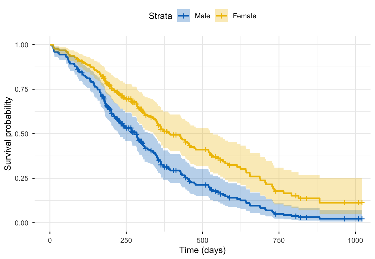
A fitted Cox model can also predict survival curves. To show how survival depends on sex while holding the other covariates fixed, build a small data frame with one row per sex (age at its mean, ph.ecog fixed at 1), pass it to survfit(), and plot with survminer’s ggsurvplot():
library(survival)library(survminer)res.cox <-coxph(Surv(time, status) ~ age + sex + ph.ecog, data = lung)# One row per sex; other covariates held at typical valuessex_df <-data.frame(sex =c(1, 2),age =rep(mean(lung$age, na.rm =TRUE), 2),ph.ecog =c(1, 1))fit <-survfit(res.cox, newdata = sex_df)ggsurvplot(fit, data = lung, conf.int =TRUE,legend.labs =c("Male", "Female"),palette ="jco", ggtheme =theme_minimal(),xlab ="Time (days)", ylab ="Survival probability")
The female curve stays above the male curve at every time point — the model’s predicted survival advantage for women, the same story the HR of 0.58 told numerically.
Report
A multivariate Cox proportional hazards model on the NCCTG lung-cancer data (n = 227, 164 deaths) showed that female sex was associated with a significantly lower hazard of death (HR = 0.58, 95% CI 0.41–0.80, p = 0.001) after adjusting for age and ECOG performance score, while a higher ECOG score was associated with a higher hazard (HR = 1.59, 95% CI 1.27–1.99, p < 0.001); age was not significant (HR = 1.01, 95% CI 0.99–1.03, p = 0.23). The overall model was significant (likelihood-ratio test p < 0.001).
NoteThe math behind the Cox model (optional)
The Cox model writes the hazard for a patient with covariates \(x_1, \dots, x_p\) as the baseline hazard\(h_0(t)\) scaled by an exponential function of the covariates:
The baseline \(h_0(t)\) is left completely unspecified (this is why Cox is called semi-parametric) — the model only estimates the coefficients \(b_i\) via the partial likelihood, which depends solely on the order in which events occur, not the baseline shape.
Each \(\exp(b_i)\) is a hazard ratio. For two patients differing only in covariate \(i\), the ratio of their hazards is constant over time:
\[
\frac{h_k(t)}{h_{k'}(t)} = \frac{h_0(t)\,e^{\sum b x}}{h_0(t)\,e^{\sum b x'}} = e^{\sum b (x - x')}
\]
The \(h_0(t)\) cancels, so the ratio does not depend on \(t\) — this is the proportional-hazards assumption: if one patient’s risk is twice another’s early on, it stays twice as high throughout. That assumption must be tested (next lesson).
Compare survival between 2+ categorical groups → log-rank test.
Model the effect of one or more covariates (categorical or continuous), adjusted for each other, with a hazard ratio per factor → Cox proportional hazards (this lesson).
Fit the Cox model yourself — change the covariates, or swap sex for a continuous predictor. The sandbox boots on first Run.
🟢 With an AI agent
Ask Prova“fit a Cox proportional hazards model on my survival data, give me the hazard ratios with 95% CIs, and tell me in plain words which factors raise or lower the risk” — it answers with survival + survminer code you can run on your own data. The runtime is the judge.Ask Prova →
Common issues
Your hazard ratios “look wrong” — check the factor coding. A Cox HR is always relative to a reference level. In lung, sex is numeric (1 = male, 2 = female), so the HR is female vs male. If your grouping variable is a factor, R uses the first level as the reference — relevel it (relevel(f, ref = "...")) so the HR compares the groups you intend.
You assumed the model is valid without testing proportional hazards. Cox results are only trustworthy if the HRs are roughly constant over time. A crossing or converging effect violates the proportional-hazards assumption and biases the HR. Always test it with cox.zph() and ggcoxzph() — see Testing the proportional hazards assumption.
Missing covariate values silently drop rows.coxph() uses complete cases by default: a single NA in any covariate removes that patient (note the multivariate model used n = 227, not 228, because one ph.ecog was missing). Check cox.model$n vs nrow(data) so you know how many patients the model actually used, and decide whether imputation is warranted.
Frequently asked questions
NoteHow do I interpret a hazard ratio in a Cox model?
The hazard ratio is a multiplicative effect on the risk of the event. HR = 1 means no effect; HR < 1 means a lower hazard (better survival) — e.g. HR = 0.59 is a 41% lower hazard; HR > 1 means a higher hazard (worse survival) — e.g. HR = 1.59 is a 59% higher hazard. Always read it with its 95% confidence interval: if the CI crosses 1, the effect isn’t statistically convincing.
NoteWhat is the difference between the Cox model and the log-rank test?
The log-rank test compares survival between categorical groups and only gives a p-value — no effect size, and no way to handle continuous predictors or adjust for confounders. The Cox model is a regression: it handles continuous and categorical predictors, estimates a hazard ratio for each, and adjusts every effect for the others in a multivariate model.
NoteWhat does HR less than 1 mean in survival analysis?
An HR below 1 means the covariate is associated with a lower hazard of the event — i.e. better survival, a good prognostic factor. For example, HR = 0.59 for female sex means women have a 41% lower hazard of death than men. An HR above 1 means a higher hazard (worse survival); HR = 1 means no effect.
NoteWhat is the proportional hazards assumption?
It is the core assumption of the Cox model: the hazard ratio between any two patients is constant over time (the survival curves are proportional and don’t cross). If a covariate’s effect grows or shrinks over follow-up — or the curves cross — the assumption is violated and the single HR is misleading. Test it with cox.zph() and ggcoxzph(); see Testing the proportional hazards assumption.
NoteWhich R packages do I need for Cox regression?
Two: survival to fit the model (coxph(), Surv(), survfit()) and survminer to visualize it (ggforest() for the hazard-ratio forest plot, ggsurvplot() for survival curves, ggcoxzph() for the PH diagnostic). Both ship the lung dataset used here.
Test your understanding
ImportantPractice
Run it. In the live cell below, fit a Cox model of survival on ph.ecog alone. Fill the blank. Is the ECOG performance score a significant predictor, and is it a good or bad prognostic factor?
Interpret. A covariate has HR = 0.70 (95% CI 0.55–0.89, p = 0.004). In plain words, what is its effect on survival, and is it statistically convincing?
NoteHint
Fill the blank with ph.ecog. The response is always Surv(time, status). To judge the effect, look at exp(coef) (the HR) and its p-value, and remember HR > 1 = higher hazard = worse survival.
NoteSolution
res.cox <-coxph(Surv(time, status) ~ ph.ecog, data = lung)summary(res.cox)#> HR (exp(coef)) ~ 1.61, p ~ 0.0001 — significant, HR > 1 = a BAD prognostic factor:#> a higher ECOG performance score is associated with a higher hazard of death (worse survival).
For question 2: HR = 0.70 means a 30% lower hazard of the event ((1 − 0.70) × 100) — a protective / good prognostic factor. It is statistically convincing because the 95% CI (0.55–0.89) lies entirely below 1 and p = 0.004 < 0.05.
TipQuick check
In a Cox model, a covariate has a hazard ratio of 1.0 with a 95% CI of 0.85–1.18. What do you conclude?
NoteShow answer
No convincing effect. HR = 1 means the covariate doesn’t change the hazard, and the confidence interval straddles 1 (it includes values both below and above), so you cannot rule out “no effect”. The covariate is not a useful predictor in this model.
Conclusion
You can now fit and interpret the Cox proportional hazards model in R: build the Surv(time, status) response, fit coxph() for one covariate (univariate) or several at once (multivariate, each adjusted for the rest), and read the full output — the hazard ratio, its 95% CI, the Wald p-value, and the global tests. On the lung-cancer data, female sex cut the hazard of death by ~42% and worse ECOG performance raised it by ~59%, while age dropped out after adjustment. The survminer ggforest() forest plot and ggsurvplot() adjusted curves turn those numbers into publication-ready figures. The one thing left to verify is whether the hazard ratios hold steady over time — the proportional-hazards assumption.
Every result on this page was produced by the code shown, run at build time against a pinned R environment — edit any block and Run to reproduce it yourself.