Repeated Measures ANOVA in R: Compare Means Across Time

Test whether the means of the same subjects differ across three or more time points — rstatix the modern way

Learn to run a one-way repeated measures ANOVA in R — the within-subjects test that compares three or more measurements taken on the same individuals. Use rstatix anova_test() for a tidy result with a ges effect size and the automatic Greenhouse-Geisser sphericity correction, check the outlier, normality and sphericity (Mauchly) assumptions, and follow up with pairwise paired t-tests on a ggpubr boxplot.

TipKey takeaways

• A one-way repeated measures ANOVA compares three or more means measured on the same subjects — the within-subjects extension of the paired t-test. Measuring the same people removes the between-subject variation, making it more powerful.
• Use anova_test(dv, wid, within) from rstatix: it returns the F-test, the ges effect size, Mauchly’s test of sphericity, and the Greenhouse-Geisser / Huynh-Feldt corrected p-values — all in one call.
• Sphericity is the key extra assumption: the variances of the differences between every pair of time points should be equal. get_anova_table() applies the Greenhouse-Geisser correction automatically when it’s violated.
• Check the assumptions: no extreme outliers (identify_outliers()) and normality per time point (shapiro_test()). If they fail, use the non-parametric Friedman test instead.
• Follow a significant result with pairwise paired t-tests (pairwise_t_test(..., paired = TRUE, p.adjust.method = "bonferroni")), drawn on a ggpubr boxplot with stat_pvalue_manual().

Introduction

A one-way repeated measures ANOVA answers a question that ordinary ANOVA can’t: did the same subjects change across three or more time points or conditions? Because every person is measured repeatedly — say, self-esteem at three points during a diet — the design is within-subjects, and the test is the extension of the paired-samples t-test beyond two measurements.

The payoff of measuring the same people is power: each subject acts as their own control, so the test removes the between-subject differences (some people are simply higher than others) and tests the within-subject change directly. This lesson runs the whole workflow the modern, pipe-friendly rstatix way — anova_test() with the dv/wid/within arguments — using the built-in datarium::selfesteem data, and shows the assumption checks (including the extra one, sphericity) that tell you whether to trust the F-test.

Note

Repeated measures hypotheses. Null: the means at all time points are equal. Alternative: at least one time-point mean differs. With exactly two time points, the repeated measures ANOVA and the paired t-test give identical results.

How repeated measures ANOVA works

Like an ordinary ANOVA it splits the variation in the outcome — but it carves out a third piece:

1. Between-subjects variance — how much subjects differ from each other overall. A repeated measures ANOVA removes this from the error term (that’s where its extra power comes from).
2. Within-subjects variance — split into the effect of the time factor (what we test) and the leftover residual (the subject × time interaction).
3. The F-statistic is the ratio of the time effect to that residual.

Because the same subjects appear at every time point, the measurements are correlated, which is why the test carries an extra assumption — sphericity — that ordinary between-subjects ANOVA doesn’t.

NoteThe math (optional)

In a within-subjects design the total variation (\(SS_T\)) is partitioned so that the subject effect (\(SS_S\)) is removed from the error term — leaving the time effect (\(SS_W\)) and the residual (\(SS_R\)):

\[SS_T = SS_S + SS_W + SS_R\]

Pulling \(SS_S\) out is exactly what gives the test its extra power — each person’s baseline level no longer inflates the error. The F-statistic for the time effect is then the ratio of the time mean square to the residual (subject × time) mean square:

\[F = \frac{MS_W}{MS_R}\]

with \(df_W = k - 1\) for \(k\) time points and \(df_R = (k - 1)(n - 1)\) for \(n\) subjects. When sphericity is violated, both degrees of freedom are multiplied by the Greenhouse-Geisser epsilon \(\hat{\varepsilon}\) before reading the p-value.

Data preparation

We use the selfesteem dataset from the datarium package — self-esteem score for 10 individuals measured at three time points (t1, t2, t3) during a diet. It arrives in wide format (one row per subject, one column per time), but rstatix needs long format (one row per measurement). We reshape it to long with base R — stacking the three time columns into one score column and a time factor — keeping id and time as factors (no extra packages needed):

library(rstatix)

data("selfesteem", package = "datarium")
head(selfesteem, 3)

# A tibble: 3 × 4
     id    t1    t2    t3
  <int> <dbl> <dbl> <dbl>
1     1  4.01  5.18  7.11
2     2  2.56  6.91  6.31
3     3  3.24  4.44  9.78

selfesteem <- data.frame(
  id    = factor(rep(selfesteem$id, times = 3)),
  time  = factor(rep(c("t1", "t2", "t3"), each = nrow(selfesteem))),
  score = c(selfesteem$t1, selfesteem$t2, selfesteem$t3)
)
head(selfesteem, 3)

  id time    score
1  1   t1 4.005027
2  2   t1 2.558124
3  3   t1 3.244241

The long table has three columns — id (the subject), time (the within-subjects factor, t1/t2/t3) and score (the outcome). Every block below rebuilds this long table so it runs on its own.

Look at the data first

Always summarize, then plot, before testing. Put numbers on the table first with rstatix get_summary_stats() — the mean and standard deviation at each time point:

library(rstatix)

data("selfesteem", package = "datarium")
selfesteem <- data.frame(
  id    = factor(rep(selfesteem$id, times = 3)),
  time  = factor(rep(c("t1", "t2", "t3"), each = nrow(selfesteem))),
  score = c(selfesteem$t1, selfesteem$t2, selfesteem$t3)
)

selfesteem %>% group_by(time) %>% get_summary_stats(score, type = "mean_sd")

# A tibble: 3 × 5
  time  variable     n  mean    sd
  <fct> <fct>    <dbl> <dbl> <dbl>
1 t1    score       10  3.14 0.552
2 t2    score       10  4.93 0.863
3 t3    score       10  7.64 1.14 

Now picture it. A ggpubr boxplot of score by time, with the overall ANOVA p-value and the pairwise paired-t brackets printed on the panel, shows the trajectory at a glance:

library(rstatix)
library(ggpubr)

data("selfesteem", package = "datarium")
selfesteem <- data.frame(
  id    = factor(rep(selfesteem$id, times = 3)),
  time  = factor(rep(c("t1", "t2", "t3"), each = nrow(selfesteem))),
  score = c(selfesteem$t1, selfesteem$t2, selfesteem$t3)
)

# Pairwise paired t-tests, positioned for the brackets
pwc <- selfesteem %>%
  pairwise_t_test(score ~ time, paired = TRUE, p.adjust.method = "bonferroni") %>%
  add_xy_position(x = "time")

res.aov <- anova_test(data = selfesteem, dv = score, wid = id, within = time)

ggboxplot(selfesteem, x = "time", y = "score", fill = "time", palette = "jco",
          xlab = "Time point", ylab = "Self-esteem score") +
  stat_pvalue_manual(pwc, hide.ns = TRUE, tip.length = 0.01) +
  labs(subtitle = get_test_label(res.aov, detailed = TRUE))

Self-esteem climbs steadily from t1 to t3, and the brackets flag which time points differ. The picture suggests a real change over the diet — let’s confirm it with the test, after the assumptions.

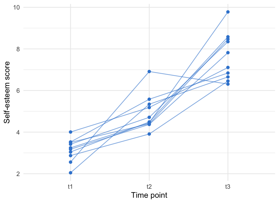
The boxplot hides the design’s real strength: the same subjects are followed over time. Connect each subject’s three measurements to see the individual trajectories — most lines climbing together is exactly the within-subject change a repeated measures ANOVA is built to detect:

library(ggpubr)

data("selfesteem", package = "datarium")
selfesteem <- data.frame(
  id    = factor(rep(selfesteem$id, times = 3)),
  time  = factor(rep(c("t1", "t2", "t3"), each = nrow(selfesteem))),
  score = c(selfesteem$t1, selfesteem$t2, selfesteem$t3)
)

ggplot(selfesteem, aes(x = time, y = score, group = id)) +
  geom_line(color = "#3a86d4", alpha = 0.6) +
  geom_point(color = "#3a86d4", size = 1.6) +
  labs(x = "Time point", y = "Self-esteem score") +
  theme_minimal()

Check the assumptions

A repeated measures ANOVA makes three assumptions worth checking (beyond independent subjects): no extreme outliers, normality of the outcome at each time point, and sphericity of the differences. The first two come before the test; sphericity is reported by the test.

No extreme outliers

identify_outliers() flags points beyond the boxplot whiskers per group — is.extreme == TRUE marks the ones that can distort the result:

library(rstatix)

data("selfesteem", package = "datarium")
selfesteem <- data.frame(
  id    = factor(rep(selfesteem$id, times = 3)),
  time  = factor(rep(c("t1", "t2", "t3"), each = nrow(selfesteem))),
  score = c(selfesteem$t1, selfesteem$t2, selfesteem$t3)
)

selfesteem %>%
  group_by(time) %>%
  identify_outliers(score)

# A tibble: 2 × 5
  time  id    score is.outlier is.extreme
  <fct> <fct> <dbl> <lgl>      <lgl>     
1 t1    6      2.05 TRUE       FALSE     
2 t2    2      6.91 TRUE       FALSE     

There were no extreme outliers. If you have one, it may be a data-entry error; you can re-run the ANOVA with and without it to gauge its influence, or use a robust ANOVA (the WRS2 package).

Normality per time point

The outcome should be approximately normal at each time point. Test it with Shapiro-Wilk per group (p > 0.05 → no departure from normal):

library(rstatix)

data("selfesteem", package = "datarium")
selfesteem <- data.frame(
  id    = factor(rep(selfesteem$id, times = 3)),
  time  = factor(rep(c("t1", "t2", "t3"), each = nrow(selfesteem))),
  score = c(selfesteem$t1, selfesteem$t2, selfesteem$t3)
)

selfesteem %>%
  group_by(time) %>%
  shapiro_test(score)

# A tibble: 3 × 4
  time  variable statistic     p
  <fct> <chr>        <dbl> <dbl>
1 t1    score        0.967 0.859
2 t2    score        0.876 0.117
3 t3    score        0.923 0.380

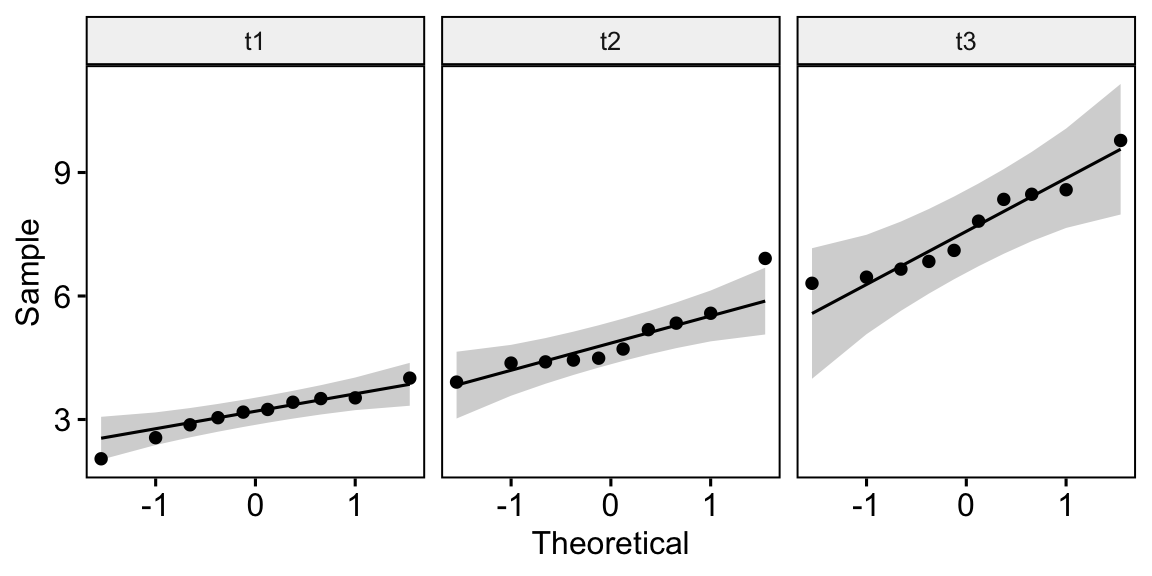
The score is normally distributed at every time point (all p > 0.05). Back it with a Q-Q plot per time point — points should hug the reference line:

library(ggpubr)
library(rstatix)

data("selfesteem", package = "datarium")
selfesteem <- data.frame(
  id    = factor(rep(selfesteem$id, times = 3)),
  time  = factor(rep(c("t1", "t2", "t3"), each = nrow(selfesteem))),
  score = c(selfesteem$t1, selfesteem$t2, selfesteem$t3)
)

ggqqplot(selfesteem, "score", facet.by = "time")

Sphericity — Mauchly’s test (handled for you)

Sphericity is the assumption unique to repeated measures designs: the variances of the differences between every pair of time points should be equal. It’s tested with Mauchly’s test of sphericity, and you don’t run it separately — anova_test() reports it automatically alongside the F-test. Crucially, when sphericity is violated, get_anova_table() applies the Greenhouse-Geisser correction automatically (adjusting the degrees of freedom), so the p-value you read is already corrected. You see all of this in the next section.

Run the repeated measures ANOVA

anova_test() takes the data plus three arguments — dv (the outcome), wid (the subject id) and within (the within-subjects factor) — and returns a list with the ANOVA, Mauchly’s test and the sphericity corrections:

library(rstatix)

data("selfesteem", package = "datarium")
selfesteem <- data.frame(
  id    = factor(rep(selfesteem$id, times = 3)),
  time  = factor(rep(c("t1", "t2", "t3"), each = nrow(selfesteem))),
  score = c(selfesteem$t1, selfesteem$t2, selfesteem$t3)
)

res.aov <- anova_test(data = selfesteem, dv = score, wid = id, within = time)
res.aov

ANOVA Table (type III tests)

$ANOVA
  Effect DFn DFd      F        p p<.05   ges
1   time   2  18 55.469 2.01e-08     * 0.829

$`Mauchly's Test for Sphericity`
  Effect     W     p p<.05
1   time 0.551 0.092      

$`Sphericity Corrections`
  Effect  GGe      DF[GG]    p[GG] p[GG]<.05   HFe      DF[HF]    p[HF]
1   time 0.69 1.38, 12.42 2.16e-06         * 0.774 1.55, 13.94 6.03e-07
  p[HF]<.05
1         *

The printout has three parts: the ANOVA table (F, DFn/DFd, p, and ges — the generalized eta-squared effect size), Mauchly’s Test for Sphericity (only shown for factors with > 2 levels, since sphericity is automatic for two), and the Sphericity Corrections (Greenhouse-Geisser GGe and Huynh-Feldt HFe epsilons with their corrected p-values).

get_anova_table() returns the single table you should report — automatically the corrected row when Mauchly’s test is significant, the standard row when it isn’t:

library(rstatix)

data("selfesteem", package = "datarium")
selfesteem <- data.frame(
  id    = factor(rep(selfesteem$id, times = 3)),
  time  = factor(rep(c("t1", "t2", "t3"), each = nrow(selfesteem))),
  score = c(selfesteem$t1, selfesteem$t2, selfesteem$t3)
)

res.aov <- anova_test(data = selfesteem, dv = score, wid = id, within = time)
get_anova_table(res.aov)

ANOVA Table (type III tests)

  Effect DFn DFd      F        p p<.05   ges
1   time   2  18 55.469 2.01e-08     * 0.829

Here self-esteem differs significantly across the three time points, F(2, 18) = 55.5, p < .0001, and ges is large (≈ 0.83) — time explains most of the within-subject variation. By Cohen’s conventions for ges, a small effect is ≈ 0.01, medium ≈ 0.06 and large ≥ 0.14, so 0.83 is exceptionally large. Mauchly’s test was non-significant, so sphericity held and no correction was needed; had it been violated, get_anova_table() would have returned the Greenhouse-Geisser-corrected line instead.

Tip

Run it on your own data. Load your wide file — mydata <- read.csv("my-file.csv") — reshape the repeated columns to long (base R reshape(), or tidyr::pivot_longer() if you use the tidyverse), make the id and time columns factors, then call anova_test(data = mydata, dv = score, wid = id, within = time).

Note

The classic base-R route. You can fit the same model with aov(score ~ time + Error(id/time), data = selfesteem) and read it with summary(). It computes the same F-test, but it does not report Mauchly’s test or apply the sphericity correction for you — the reason anova_test() is the lead here. Use base R only when you need the raw aov object.

Choosing the sphericity correction: Greenhouse-Geisser vs Huynh-Feldt

When sphericity is violated you correct the F-test, and the Sphericity Corrections block gives you two options — Greenhouse-Geisser (GGe) and Huynh-Feldt (HFe). Both work through epsilon (ε), a number that measures how far the data depart from sphericity: ε = 1 means no departure at all, and the further ε falls below 1, the worse the violation. Each correction multiplies the degrees of freedom by ε before the p-value is read — a smaller ε shrinks the degrees of freedom more, making the test more conservative. (The F-statistic itself never changes; only the degrees of freedom and the p-value do.)

The two estimators trade off in opposite directions: Greenhouse-Geisser is the more conservative (it can over-correct when the true ε is close to 1), while Huynh-Feldt is the less conservative (it can under-correct when ε is small). The standard rule of thumb picks between them by the Greenhouse-Geisser epsilon:

• ε < 0.75 → use the Greenhouse-Geisser correction (the safer choice under a strong violation).
• ε > 0.75 → use the Huynh-Feldt correction (Greenhouse-Geisser is too conservative here).

This 0.75 threshold is the classic recommendation of Girden’s ANOVA: Repeated Measures monograph (Girden, E. R. (1992). ANOVA: Repeated Measures. Newbury Park, CA: Sage), and it is what most statistics packages implement.

By default get_anova_table() uses correction = "auto": it applies the Greenhouse-Geisser correction when Mauchly’s test is significant and leaves the table uncorrected when it isn’t. To follow the ε rule yourself, pass correction explicitly — "GG" (Greenhouse-Geisser), "HF" (Huynh-Feldt) or "none" (the uncorrected F-test):

library(rstatix)

data("selfesteem", package = "datarium")
selfesteem <- data.frame(
  id    = factor(rep(selfesteem$id, times = 3)),
  time  = factor(rep(c("t1", "t2", "t3"), each = nrow(selfesteem))),
  score = c(selfesteem$t1, selfesteem$t2, selfesteem$t3)
)

res.aov <- anova_test(data = selfesteem, dv = score, wid = id, within = time)

get_anova_table(res.aov, correction = "GG")     # Greenhouse-Geisser

ANOVA Table (type III tests)

  Effect  DFn   DFd      F        p p<.05   ges
1   time 1.38 12.42 55.469 2.16e-06     * 0.829

get_anova_table(res.aov, correction = "HF")     # Huynh-Feldt

ANOVA Table (type III tests)

  Effect  DFn   DFd      F        p p<.05   ges
1   time 1.55 13.94 55.469 6.03e-07     * 0.829

get_anova_table(res.aov, correction = "none")   # uncorrected F-test

ANOVA Table (type III tests)

  Effect DFn DFd      F        p p<.05   ges
1   time   2  18 55.469 2.01e-08     * 0.829

Compare the three rows. The uncorrected test keeps the full degrees of freedom (DFn = 2, DFd = 18); Greenhouse-Geisser multiplies both by its epsilon (ε ≈ 0.69 here) down to 1.38 and 12.42, and Huynh-Feldt by its slightly larger epsilon (ε ≈ 0.77) down to 1.55 and 13.94. Smaller degrees of freedom read the same F = 55.5 against a stricter reference, so the p-value climbs from 2e-08 (uncorrected) to 2e-06 (GG) — still overwhelmingly significant because the effect is huge. On a borderline result the choice of correction can flip the verdict, which is exactly why the ε rule matters. Note that here the Greenhouse-Geisser ε (0.69) sits below 0.75, so the rule would favour the Greenhouse-Geisser line if you were correcting — but Mauchly’s test was non-significant, so "auto" reports the uncorrected table.

Post-hoc: which time points differ?

A significant omnibus test says some time-point mean changed — to find which pairs, run pairwise paired t-tests between the time levels, with a multiple-comparisons correction (bonferroni):

library(rstatix)

data("selfesteem", package = "datarium")
selfesteem <- data.frame(
  id    = factor(rep(selfesteem$id, times = 3)),
  time  = factor(rep(c("t1", "t2", "t3"), each = nrow(selfesteem))),
  score = c(selfesteem$t1, selfesteem$t2, selfesteem$t3)
)

pwc <- selfesteem %>%
  pairwise_t_test(
    score ~ time, paired = TRUE,
    p.adjust.method = "bonferroni"
  )
pwc

# A tibble: 3 × 10
  .y.   group1 group2    n1    n2 statistic    df         p   p.adj p.adj.signif
* <chr> <chr>  <chr>  <int> <int>     <dbl> <dbl>     <dbl>   <dbl> <chr>       
1 score t1     t2        10    10     -4.97     9   7.72e-4 2.32e-3 **          
2 score t1     t3        10    10    -13.2      9   3.34e-7 1.00e-6 ****        
3 score t2     t3        10    10     -4.87     9   8.86e-4 2.66e-3 **          

Each row is one pair of time points. Read p.adj (the Bonferroni-adjusted p-value) to see which comparisons are significant — here every pairwise difference is, so self-esteem rose significantly at each step of the diet. The paired = TRUE argument is essential: it pairs each subject’s measurements, matching the within-subjects design.

Tip

Why paired? Because the same subjects are measured at every time point, an unpaired t-test would throw away the pairing and lose the design’s power. Always pass paired = TRUE for a within-subjects post-hoc.

Report the result

A publication-style write-up pulls the omnibus result, the effect size and the significant pairwise comparisons into one statement — for example:

A one-way repeated measures ANOVA showed that self-esteem differed significantly across the three time points, F(2, 18) = 55.5, p < .0001, generalized η² = 0.83. Pairwise paired t-tests with a Bonferroni adjustment found every pair significantly different (all p.adj < .05), with self-esteem increasing from t1 to t2 to t3.

If Mauchly’s test had been significant you’d add a sphericity note — e.g. “the assumption of sphericity was violated (Mauchly’s W, p < .05), so the degrees of freedom were corrected with the Greenhouse-Geisser estimate” — and quote the corrected F and degrees of freedom.

Try it live

Run the full workflow end to end on the selfesteem data. Edit the columns, the dataset or the post-hoc method and re-run; the sandbox boots on first Run.

🟢 With an AI agent

Ask Prova “I measured the same subjects at three time points — run a repeated measures ANOVA on my data, check sphericity, and tell me which time points differ” — it answers with rstatix code you can run on your own data, then helps you read the F-test, the sphericity correction and the paired post-hoc table. The runtime is the judge. Ask Prova →

Common issues

anova_test() errors with “wid” or duplicate values. Each subject must appear once per level of the within factor, and wid must identify the subject. Make sure you reshaped to long format and that id is a factor — a numeric id or missing measurements break the design.

There’s no Mauchly’s test or sphericity correction in the output. Sphericity only applies when the within factor has more than two levels — with exactly two time points it holds automatically, so rstatix omits it. That’s expected, not a bug.

My post-hoc pairs look too significant / not paired. Check you passed paired = TRUE to pairwise_t_test(). Without it you run unpaired t-tests, which ignore the within-subjects pairing, lose power, and don’t match the ANOVA you reported.

Frequently asked questions

NoteWhat is a repeated measures ANOVA?

A repeated measures ANOVA tests whether the means of three or more measurements taken on the same subjects differ — for example the same people measured at three time points. Because every subject is their own control, it removes the between-subject variation and is more powerful than comparing independent groups. In rstatix: anova_test(data = mydata, dv = score, wid = id, within = time).

NoteWhat is the difference between a repeated measures ANOVA and a one-way ANOVA?

A one-way (between-subjects) ANOVA compares different, independent groups; a repeated measures (within-subjects) ANOVA compares the same subjects measured several times. The repeated measures design removes each subject’s baseline level from the error term, so it detects within-subject change with more power — but it adds the sphericity assumption that between-subjects ANOVA doesn’t have.

NoteWhat is sphericity, and what is Mauchly’s test?

Sphericity means the variances of the differences between every pair of within-subject levels are equal — the repeated measures version of equal variance. Mauchly’s test checks it; a significant result (p < 0.05) means sphericity is violated. rstatix’s anova_test() reports Mauchly’s test automatically and, when it’s violated, get_anova_table() applies the Greenhouse-Geisser correction to the degrees of freedom for you.

NoteWhich post-hoc test should I use after a repeated measures ANOVA?

Use pairwise paired t-tests between the within-subject levels, with a multiplicity correction: pairwise_t_test(score ~ time, paired = TRUE, p.adjust.method = "bonferroni"). The paired = TRUE argument is essential — it respects the within-subjects design. Run the post-hoc only after a significant omnibus test.

NoteWhat if my data isn’t normal or has extreme outliers?

If normality fails at one or more time points, or you have extreme outliers you can’t justify, use the non-parametric Friedman test — the rank-based alternative to the one-way repeated measures ANOVA — followed by pairwise Wilcoxon signed-rank tests. For outliers driven by errors, fix or remove them; to keep them, a robust ANOVA (the WRS2 package) is an option.

Test your understanding

ImportantPractice

1. Run it. In the live cell below, fill the blanks to run the repeated measures ANOVA of score by time on the selfesteem data, then print the report-ready table. Is the change across time significant?
2. Conceptual. Mauchly’s test in your output is significant (p < 0.05). Which row of the ANOVA should you report, and what has the software done to your degrees of freedom?

NoteHint

The outcome is score, the subject identifier is id, and the within-subjects factor is time. Read the p column of get_anova_table() for significance. For question 2, recall what Mauchly’s test checks and what get_anova_table() does when it’s violated.

NoteSolution

library(rstatix)
data("selfesteem", package = "datarium")
selfesteem <- data.frame(
  id    = factor(rep(selfesteem$id, times = 3)),
  time  = factor(rep(c("t1", "t2", "t3"), each = nrow(selfesteem))),
  score = c(selfesteem$t1, selfesteem$t2, selfesteem$t3)
)

res.aov <- anova_test(data = selfesteem, dv = score, wid = id, within = time)
get_anova_table(res.aov)
#> F(2, 18) = 55.5, p < .0001  → highly significant change across time.

For question 2: a significant Mauchly’s test means sphericity is violated, so you report the sphericity-corrected row — get_anova_table() returns it automatically. The software multiplies the degrees of freedom (DFn, DFd) by the Greenhouse-Geisser epsilon, lowering them and making the test more conservative.

Which test when?

Pick the test from your design, not the other way around:

• Three or more repeated measurements on the same subjects → one-way repeated measures ANOVA (this lesson).
• Exactly two time points on the same subjects → the paired t-test — the repeated measures ANOVA reduces to it.
• Independent groups (different subjects per condition) → the between-subjects one-way ANOVA.
• Normality or sphericity badly violated → the non-parametric Friedman test, the rank-based alternative to the repeated measures ANOVA.

Conclusion

You can now run and interpret a one-way repeated measures ANOVA in R the tidy rstatix way: reshape wide data to long with id and time as factors, then anova_test(dv = score, wid = id, within = time) for the F-test, the ges effect size, and the automatic sphericity handling. Check the assumptions — no extreme outliers (identify_outliers), normality per time point (shapiro_test), and sphericity (Mauchly, corrected by get_anova_table()) — read the omnibus F-test, then follow a significant result with pairwise paired t-tests. When the assumptions fail, the non-parametric Friedman test is the fallback.

Related lessons

• One-way ANOVA in R — the between-subjects version, for independent groups. · Mixed ANOVA — combine a within-subjects and a between-subjects factor. · Friedman test — the non-parametric alternative when normality fails.
• Go further: The ANOVA family · Biostatistics

Was this page helpful?

Prove you can do it. Master the whole ANOVA in R series — track your path, build projects, and earn a certificate.

Start free →

Go Pro — unlimited Prova on your own data and a verifiable certificate that proves the skill.

from $15/mo billed yearly

Go Pro →

✓ You're Pro — keep going. The runtime is the judge.

Ready to level up?

Prove it — earn the ANOVA & Multi-Group Comparisons certificate.Take the assessment →Try this on your own data with Prova — the runtime is the judge.Open Prova →

Get new R & Python lessons by email

Practical, reproducible, no spam. Unsubscribe anytime.

Double opt-in. We never share your email.

Share this pageXLinkedInRedditHN

Note

Every result on this page was produced by the code shown, run at build time against a pinned R environment — edit any block and Run to reproduce it yourself.